The computation of early dipmeter data has been handled in one of three general ways: manual processing, combination of manual and computer processing, and total computer processing. Manual correlation and computation methods were developed first and there are several different methods of doing the work. The dipmeter curves must first be correlated; this may be done by slipping a print of a log under the film used to make the print and measuring the depth displacement between peaks and valleys on the curves. Pad number one is used as a reference to measure displacements to each of the other curves. Another method of curve correlation uses an optical comparator, a system of mirrors and lenses which allow the user to optically lay one curve over another and shift it up and down. The amount of shift is measured mechanically on a dial and is recorded as the displacement. After these correlations have been made, the azimuth of the number one electrode, the borehole deviation angle, the relative bearing, and the borehole diameter from the calipers are recorded. This information, plus the depth, is necessary to compute the dip angle and dip direction of a point referenced to magnetic north. Because true dip is referenced to true north, we must also account for magnetic declination of the region. Mathematical formulas to solve this geometric puzzle are given later in this Chapter. The manual calculation of dip magnitude and direction with the above information was made in several ways: by using a calculator and trigonometric tables, a scientific programmable calculator (after 1970) with trig functions, a mathematically derived physical computing device (in other words, an analog computer), or stereographic nets, the latter being the most common manual method used in the past. A very small amount of hand calculator work is still done today. Another method of dipmeter computation utilized manual correlation and computer reduction of the data. This type of processing was originally developed to minimize turnaround time and to allow the tedious, time consuming computation and plotting of results to be performed by a digital computer. This may still be done today for re-computation of continuous dipmeters recorded on paper, or on 7 track digital tapes (which are unreadable by most modern computers) for which the paper records are still available. The most recently developed system of computation is computer correlation and calculation from data on digital magnetic tape. The data from the magnetic tape is entered into a digital computer and processed. In the correlation program, the digital information representing the dipmeter curves is stored in memory and the data from one trace is compared to the other traces to determine the vertical displacement between the traces. After these displacements are calculated, the tool orientation information is used to compute the actual formation dips. The standard correlation process is performed by a mathematical function called cross-correlation, in which the offset distance between events on two curves are found. The distance between the center and the maximum amplitude on the correlagram indicates the displacement between the two curves. The offsets for all curve pairs are then adjusted to obtain the offsets relative to the center of the correlation interval. More exotic forms of correlation, some based on pattern recognition theory, are used in the newer programs. The length of the portion of the curve being correlated is called the correlation interval, correlation length, or correlation window. Correlation interval is usually between one and four feet, but can be smaller or larger. The correlation is calculated at regular intervals along the log. The distance between correlations is called the step distance and is usually 1/2 to 1/4 of the correlation interval. One dip value is calculated at the center of each correlation window, and the dip value is plotted at each step distance.
Dipmeter computation definitions
The number of dips computed from computer processed logs can be any density required for a particular purpose. For structural analysis, normal densities range from one computation every one or two feet to one computation every ten feet. In those instances where additional information is required, such as for stratigraphic analysis, points as close as every few inches can be computed. The usual way to describe these parameters is in the form CORR x STEP x ANGLE. For example a 4 x 1 x 45 process uses a 4 foot correlation, a 1 foot step, with a 45 degree search angle. The recommended defaults for dipmeter processing are: Low angle structural dip: 4 x 2 x 45 eg: normal or reverse faults, folds High angle structural dip: 8 x 4 x 80 eg: overthrust faults, recumbent folds Sand body stratigraphic dip: 2 x 1 x 30 eg: beach, bar, channel, drape Complex stratigraphic dip: 1 x 0.5 x 30 eg: submarine fan, scree slope, turbidite A
fourth parameter is sometimes used to indicate that the program
can search farther up the curve if no correlation is found. This
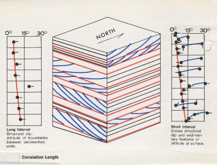
is shown as: The effect of a shorter correlation interval is shown below, where only regional dip is found in the long interval case, and stratigraphic dip is superimposed on the regional when a short interval is used.
The problem with dip determination by cross-correlation is that it does average all dips found in the correlation interval. If both structural and stratigraphic dips are present, the average may not reflect either of them correctly, regardless of the correlation interval. Regional dip is therefore usually chosen in a nearby shale or bedded carbonate thick enough to give an accurate result, without interference from stratigraphic events. Many dipmeters have been computed with inappropriate parameters and could be improved by re-computation with a better choice of values. The defaults shown above are just starting points. In particular, parameters for steeply deviated holes may need considerable experimentation and variation throughout the hole. To compute the displacements between the wiggles on a three curve continuous dipmeter, we could correlate at each computation level, defined by the correlation length, a segment of curve 1 with curve 2 first, and then correlate a segment of curve 2 with curve 3. The two displacements found would be sufficient to determine the dip. However, we might just as well have correlated curves 2 and 3 then curves 3 and 1, or curves 3 and 1 and then 1 and 2. All three combinations of displacement pairs should in theory define the same bedding plane, and the same dip. If they do not, a closure error exists. In manual correlations, one could correlate three pairs, determining three displacements. For perfect closure, the algebraic sum of the displacements must be zero. Usually, because of the inaccuracy of the optical comparator, a small closure error existed. This error could then be distributed among the three displacements as a small correction before final determination of the dip. In practice, this was an onerous task, and two pairs were often picked with no attempt to determine closure error. In automatic correlations, two kinds of closure errors can occur: small ones due to minor variations in shape between the three curves, and large errors. Small errors are handled as for manual computation. When a large error exists, it is because at least one of the correlations is in error - the same geological event is not being picked on all three pairs. In manual correlation, a large error was usually fixed by re-picking one of the correlated curves. For an automatic computation, we have to choose between three possible computable dips, only one of which may be correct. There are no strong mathematical rules to choose the correct dip. If closure error is large, the usual procedure is to compute no result and display no dip arrow. The
three arm tool is also vulnerable to adverse hole conditions.
If one curve degenerates, for instance when one pad fails to make
a good contact with the borehole wall, the computation of dip
cannot be made at all. This happens often in deviated holes or
in out-of-round holes, resulting in more intervals with no result. |
|
||
|
Page Views ---- Since 01 Jan 2015
Copyright 2023 by Accessible Petrophysics Ltd. CPH Logo, "CPH", "CPH Gold Member", "CPH Platinum Member", "Crain's Rules", "Meta/Log", "Computer-Ready-Math", "Petro/Fusion Scripts" are Trademarks of the Author |
|||

|
||
| Site Navigation | DIPMETER PROCESSING THREE ARM DIPMETERS | Quick Links |
 In
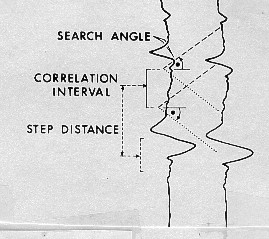
order to determine how far up and down each adjacent curve the
correlation is to be performed, a search angle is defined. In
moderate structural dip the search angle is usually 45 degrees,
but if expected dips are low, the angle can be reduced to
eliminate noise, or spurious dips caused by erratic wiggles on
the curves. Some computer programs use a search length instead
of a search angle. In steep dips, a higher search angle is
required. These terms are illustrated at the right.
In
order to determine how far up and down each adjacent curve the
correlation is to be performed, a search angle is defined. In
moderate structural dip the search angle is usually 45 degrees,
but if expected dips are low, the angle can be reduced to
eliminate noise, or spurious dips caused by erratic wiggles on
the curves. Some computer programs use a search length instead
of a search angle. In steep dips, a higher search angle is
required. These terms are illustrated at the right.