DIPS FROM RESISTIVITY Image log (MICROSCANNER)
With FMS and FMI data in the form of a digital image, several image processing operations can be used to improve the overall quality of the imagery. For example, systematic variations between electrode responses are normalized, and dynamic or user controlled gray scale compensation is used to enhance local image contrast and improve the fine image detail. An example is shown in the next Section. Stretching, squeezing, or clipping of the colour spectrum, or mapping of the gray scale to colours, are common processing functions. Edge enhancement or directional filters can also be applied to sharpen various features seen on the images.

The FMS Image Examiner is an interactive computer program for image enhancement and dip calculation using data from the formation microscanner. The program provides the analyst with the tools to manipulate the image in many ways, one of which is to calculate dip angle and direction. A simple example will illustrate the technique. The illustration below shows the colour image from two passes of the microscanner. Dark colours represent shale and light colours are sandstone. Notice the detailed depth scale (shown in meters). The white area is very high resistivity, probably a limestone stringer.

Image Examiner showing tight streak (white) in sand shale sequence on formation
microscanner images

By using a mouse to digitize bedding planes such as the thin shale laminations and the boundaries of the limestone layer, the program fits a sine wave to the points. The sine wave represents a plane slicing through the borehole, and its dip and direction can be calculated. These are displayed on the right edge of the screen.

It is obvious that the sine waves shown within the white (limestone) layer could not have been digitized from this image. In fact, the image scale was enlarged, then the colour scale was shifted to provide greater resolution in the high resistivity band, turning previously bright colours into black, and white into distinguishable colours. Now the bedding planes can be digitized and dips computed.

Expanded vertical scale image of tight streak (white) on formation microscanner

Expanded colour scale image of tight streak (light brown) on formation microscanner

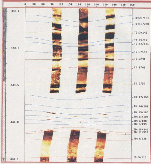
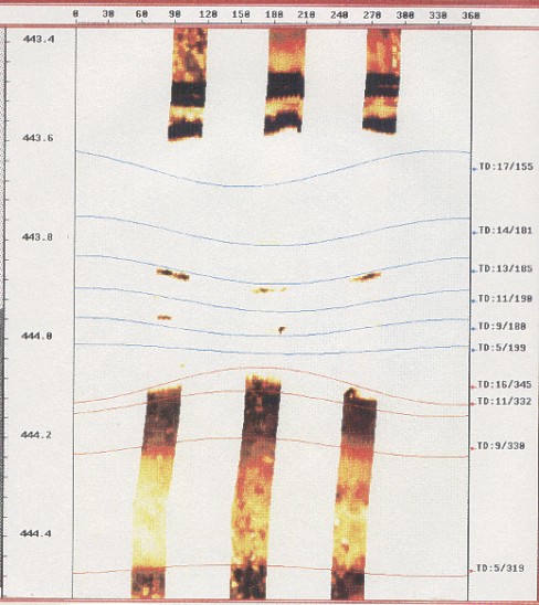
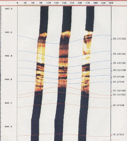
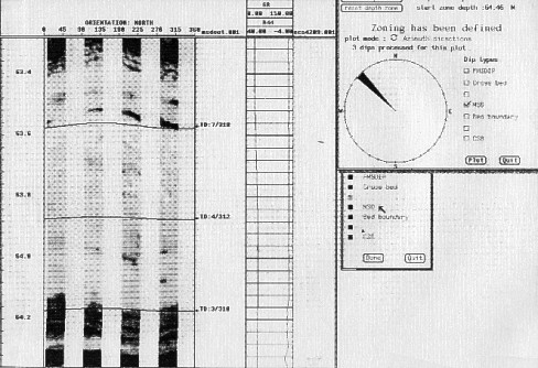
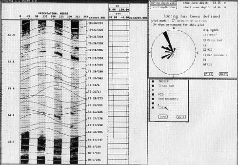
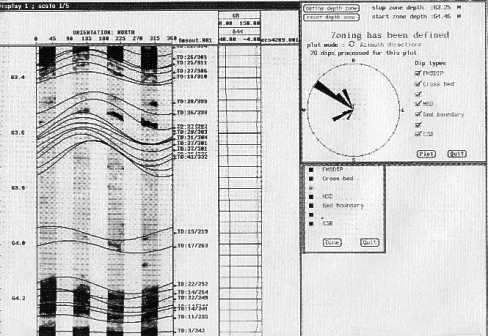
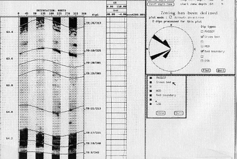
Dips can also be computed automatically by the same methods as used for the stratigraphic high resolution dipmeter. MSD, CSB, LOC, FMS, and handpicked dips over the same interval are demonstrated in the next several illustrations. Each plot has entirely different dip results, emphasizing the need to understand the different dip calculation methods. In particular, the MSD dips in a strongly cross bedded formation suffer badly from the averaging calculation. Compare the MSD with the CSB dips on the images. It is clear that MSD dips do not follow the bed boundaries very well and underestimate dip angle at the sand top and base by 7 to 10 degrees.

MSD dips picked from formation microscanner

 CSB dips picked from formation microscanner

FMS dips picked from formation microscanner

Hand picked dips picked from formation microscanner

The FMS dips use a different form of correlation, so they honour the bed boundaries even better. Computed dips are even steeper than CSB and much steeper than the MSD, indicating the relative degree of averaging being done by the program. The hand picked data is probably the best result, but it is labor intensive. It takes about half a day to compute all FMS dips over a 300 foot interval, delete all unwanted dips manually, and pick additional dips not found in the original computation.

You should appreciate these differences when using any dipmeter. Any form of best fit or averaged dip will probably underestimate dip angle unless some very dominant bed boundary exists that will swamp all others. The assumption made by the programmers is that major bed boundaries do this, but as you can see from the illustrations, this is not always true. If you can afford it, run FMS or televiewer images to help interpret dipmeter arrow plots. Since the vast majority of existing dipmeters cannot be augmented by FMS, BEWARE of averaged results.

The borehole televiewer, an ultrasonic borehole imaging tool, has much resolution than the dipmeter based imaging tools. As a result, only the largest dip and bedding features can be seen. It is used mostly for fracture identification.