|
 Total Organic CARBON (TOC) BASICS
Organic carbon
in the form of kerogen is the remnant of ancient life preserved in
sedimentary rocks, after degradation by bacterial and chemical
processes, and further modified by temperature, pressure, and time.
The latter step, called thermal maturation, is a function of burial
history (depth) and proximity to heat sources. Maturation provides
the chemical reactions needed to give us gas, oil, bitumen,
pyrobitumen, and graphite (pure carbon) that we find while drilling
wells for petroleum.
Organic
carbon is usually associated with shales or silty shales,
but may be present in relatively clean siltstone, sandstone, and carbonate rocks.
A source rock is a fine grained sediment
rich in organic matter that could generate crude oil or natural gas
after thermal alteration of kerogen in the Earth's crust. The oil or
gas could then migrate from the source rock to more porous and
permeable sediments, where ultimately the oil or gas could
accumulate to make a commercial oil or gas reservoir.
If a source rock has
not been exposed to temperatures of about 100 °C, it is termed a
potential source rock. If generation and expulsion of oil or gas
have occurred, it is termed an actual source rock. The terms
immature and mature are commonly used to describe source rocks and
also the current state of the kerogen contained in the rock.
Total organic
carbon (TOC) as measured by laboratory techniques historically has
been used to assess the quality of source rocks,
but now is widely used to help evaluate some unconventional reservoirs
(reservoirs that are both source and productive).
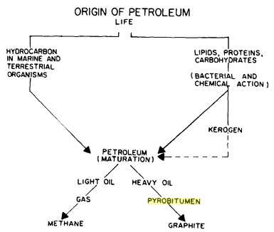  Pathways that
convert living organisms to organic carbon, from "Bitumens,
Asphalts, and Tar Sands" by
George V.
Chilingar,
Teh Fu Yen, 1978. Pathways that
convert living organisms to organic carbon, from "Bitumens,
Asphalts, and Tar Sands" by
George V.
Chilingar,
Teh Fu Yen, 1978.
In the
lab, it is relatively easy to distinguish kerogen from hydrocarbons:
kerogen is insoluble in organic solvents, oil and bitumen are
soluble. Pyrobitumen is not soluble but its hardness is used to
identify it from kerogen.
Graphite is evident on resistivity logs because of the very
low resistivity; all other forms of organic carbon are resistive.
Organic
carbon has a density near that of water, so it looks like fsporosity
to conventional porosity logs. High resistivity with some apparent porosity on a log
analysis is a good indicator of organic carbon content OR
ordinary hydrocarbons OR both.
Some more definitions are in order. All hydrocarbons are composed of
organic matter (OM), posibly with inorganic impurities. Kerogen and
coal are called primary organic matter as they were deposited during
sedimentation. Gas, oil, bitumen, and pyrobitumen are called
seccondary organic matter as they were formed in place in a source
rock and may have migraated from there to another reserervoir rock.
Kerogen has been associated historically with source rocks but has
gained more notice recently as the source of hydrocarbons in
so-called gas shale and oil shale (unconventional) reservoirs.
Kerogen is the source of oil or gas in the free porosity and can
also hold producible gas within its structure in the form of
adsorbed gas. Some reservoirs that have been treated or described as
gas shale or oil shale have little or no kerogen (tight gas or tight
oil reservoirs). Some of tight gas plays may have bitumen or
pyrobitumen, instead of kerogen. Pyrobitumen can hold adsorbed gas
in nano- or micro-porosity, similar to kerogen.
For example, where the generated hydrocarbons have largely remained
within the source rock, as in the Barnett Shale, the organic matter
will be a mixture of kerogen and pyrobitumen. However in other tight
gas plays (Montney, Marcellus), petrographic analysis indicates that
pyrobitumen is the dominant, sometimes the only, form of organic
solid, and therefore the primary reservoir for adsorbed gas.
Despite the genetic difference in origin of kerogen and pyrobitumen,
there is a tendency to classify all shale organic matter as kerogen
in geochemical analyses, due to the lack of petrographic or SEM work
which would clarify the situation.
TYPES OF KEROGEN
Organic
material can be classified according to the source of
the material, as shown below.
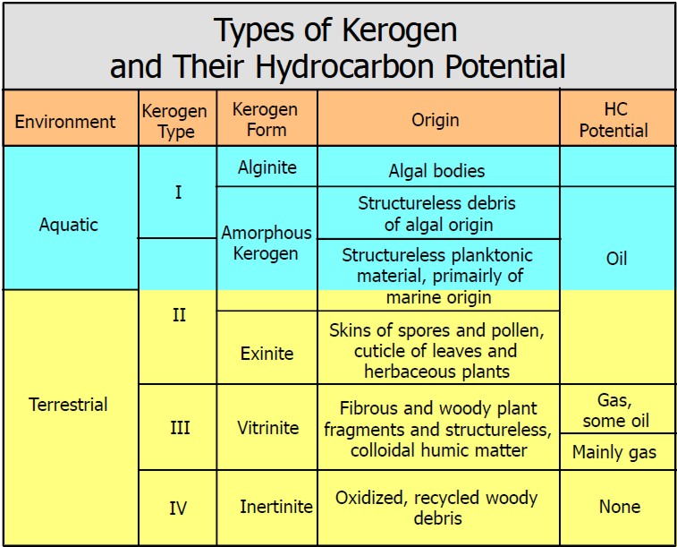
Origin, type, source, and
hydrocarbon potential of different kerogens.
Organic content in gas shales is usually Type II,
as opposed to coals, which contain mostly Type III
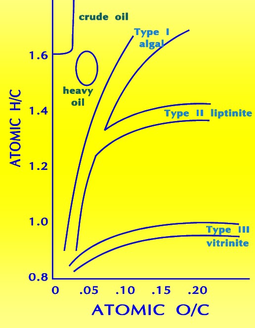 The
most commonly utilized scheme for classifying organic matter in
sediments is based on the relative abundance of elemental carbon,
oxygen, and hydrogen plotted graphically as the H/C and O/C ratio on
a so called Van Krevelen diagram. The
most commonly utilized scheme for classifying organic matter in
sediments is based on the relative abundance of elemental carbon,
oxygen, and hydrogen plotted graphically as the H/C and O/C ratio on
a so called Van Krevelen diagram.
The classic Van Krevelen diagram 
Rather than plot the elemental ratios it is common to plot indices
determined by a pyrolysis technique referred to as Rock Eval. In the
pyrolysis techniques two indices are determined: the Hydrogen Index
(HI) which is milligrams of pyrolyzable hydrocarbons divided by TOC
and the Oxygen Index (OI) which is milligrams of pyrolyzable organic
carbon dioxide divided by TOC.
Cross-plots of both elemental H/C and O/C ratios or of HI and OI are
utilized to discriminate four ‘fields’ which are referred to as
Types I, II, III, and IV kerogen.
Type I kerogen is hydrogen rich (atomic H/C of 1.4 to 1.6: HI of >
700) and is derived predominantly from zooplankton, phytoplankton,
micro-organisms (mainly bacteria) and lipid rich components of
higher plants (H/C ratio 1.7 to 1.9).
Type II kerogen is intermediate in composition (H/C ≈ 1.2: HI ≈ 600)
and derived from mixtures of highly degraded and partly oxidized
remnants of higher plants or marine phytoplankton.
Type III kerogen is hydrogen poor (H/C ratio 1.3 to 1.5) and oxygen
rich and is mainly derived from cellulose and lignin derived from
higher plants.
Type IV kerogen is hydrogen poor and oxygen rich and essentially
inert. This organic matter is mainly derived from charcoal and
fungal bodies. Type IV kerogen is not always distinguished but is
grouped with Type III.
The different types of organic matter are of fundamental importance
since the relative abundance of hydrogen, carbon, and oxygen
determines what products can be generated from the organic matter
upon diagenesis. Since coal is comprised predominantly of Type III
kerogen, there is little liquid hydrogen generating capacity. If the
coal includes abundant hydrogen rich components (such as spores,
pollen, resin, waxes - Type I or II), it will generate some liquid
hydrocarbons. Although not common, some oil deposits are thought to
be sourced by coals.
Note: Portions of the above
Section, and the next Section, were taken verbatim (with moderate
editing) from CBM Solutions reports.
Analyzing TOC IN THE LABORATORY
The total
organic carbon content of rocks is obtained by heating the
rock in a furnace and combusting the organic matter to
carbon dioxide. The amount of carbon dioxide liberated is
proportional to the amount of carbon liberated in the
furnace, which in turn is related to the carbon content of
the rock. The carbon dioxide liberated can be measured
several different ways. The most common methods use a
thermal conductivity detector or infrared spectroscopy.
Many source rocks also include inorganic sources of carbon
such as carbonates and most notably calcite, dolomite, and
siderite. These minerals break down at high temperature,
generating carbon dioxide and thus their presence must be
corrected in order to determine the organic carbon content.
Generally, the amount of carbonate is determined by acid
digestion (normally 50% HCl) and the carbon dioxide
generated is measured and then subtracted from the total
carbon dioxide to obtain the organic fraction.
Total organic
carbon is often taken to mean the same thing as kerogen, but this is
not the case. Kerogen is made up of oxygen, nitrogen, sulphur, and
hydrogen, in addition to carbon. The standard pyrolysis lab
procedure measures only the carbon, so total organic carbon excludes
the other elements.
About 80% of a typical kerogen (by weight) is carbon, so the weight
fraction of TOC is 80% of the kerogen weight. The factor is
lower for less mature and higher for more mature kerogen:
1: Wtoc = Wker * KTOC
OR 2: Wker = Wtoc / KTOC
Where:
Wtoc = weight fraction of organic carbon
Wker = weight fraction of kerogen
KTOC = kerogen correction factor - range = 0.68 to 0.90, default 0.80
If
pyrobitumen, which cannot be removed by solvents, is known or
supected, a petrogtaphic or SEM study needs to be done to quantify
non-kerpgen organic matter. The kerogen content can then be reduced
by an appropriate amount.
Another
lab procedure, called RockEval, burns both hydrogen and carbon, so
the data needs to be calibrated to the standard method by performing
a chemical analysis on the kerogen. Typically the organic carbon
needs to be reduced by about 10% (the weight of the hydrogen burned)
to match the standard method.
Rock Eval is the trade name for a set of equipment used in the lab
to measure organic content of rocks, as well as other properties of
the organics that help to identify the kerogen type. Rock-Eval combusts
a crushed sample of rock at 600ºC. Refractory organic matter
such as inertinite does not combust readily at 600ºC so most coal
samples yield Rock-Eval measured TOC values much lower than actual
values because of incomplete combustion. Rock-Eval is not
recommended for use with coals or source rocks with significant
amounts of Type III and IV kerogen.
A rock sample is crushed finely enough so that 85% falls through a
75 mesh screen. Approximately 100 mg of sample is loaded into a
stainless steel crucible capped with a micro mesh filter. To ensure
accuracy, standard samples are loaded at the beginning and end of
the run. Any drift in data can be detected and the samples rerun if
necessary.
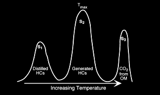
The analyzer consists of a flame ionization detector and two IR
detector cells. The free hydrocarbons (S1) are determined from an
isothermal heating of the sample at 340 degrees Celsius. These
hydrocarbons are measured by the flame ionization detector. The
temperature is then increased from 340 to 640 degrees Celsius.
Hydrocarbons are then released from the kerogen and measured by the
flame ionization detector creating the S2 peak. The temperature at
which S2 reaches its maximum rate of hydrocarbon generation is
referred to as Tmax. The CO2 generated from the oxidation step in
the 340 to 580 degrees Celsius is measured by the IR cells and is
referred to the S3 peak.
 Measured results from a typical Rock Eval study will contain: Measured results from a typical Rock Eval study will contain:
TOC% - Weight percentage of organic carbon
S1 = amount of free hydrocarbons in sample (mg/g)
S2 = amount of hydrocarbons generated through thermal
cracking (mg/g) –
provides the quantity of
hydrocarbons that the
rock has the potential to
produce through diagenesis.
S3 = amount of CO2 (mg of CO2/g of rock) - reflects the amount of oxygen
in the oxidation step.
Ro = vitrinite reflectance (%)
Tmax = the temperature at which maximum rate of
generation
of hydrocarbons occurs.
Calculated results include:
Hydrogen index
1: HI = 100 * S2 / TOC%
Oxygen index
2: OI = 100 * S3 / TOC%
Production index
3: PI = S1 / (S1 + S2)
|
Depth (m) |
TOC |
SRA |
Tmax |
Meas. |
HI |
OI |
S2/S3 |
S1/TOC*100 |
PI |
|
Top |
S1 |
S2 |
S3 |
(°C) |
% Ro |
|
X025 |
1.35 |
0.05 |
1.72 |
0.63 |
444 |
|
128 |
47 |
3 |
4 |
0.03 |
|
X040 |
1.18 |
0.05 |
1.65 |
0.57 |
443 |
|
140 |
49 |
3 |
4 |
0.03 |
|
X050 |
0.83 |
0.03 |
1.31 |
0.55 |
443 |
|
158 |
66 |
2 |
4 |
0.02 |
|
X065 |
0.80 |
0.04 |
1.00 |
0.58 |
440 |
|
126 |
73 |
2 |
5 |
0.04 |
|
X075 |
0.75 |
0.05 |
1.04 |
0.72 |
438 |
|
138 |
96 |
1 |
7 |
0.05 |
|
X090 |
1.04 |
0.09 |
2.52 |
0.29 |
452 |
|
241 |
28 |
9 |
9 |
0.03 |
|
X110 |
1.02 |
0.05 |
1.16 |
0.56 |
441 |
|
114 |
55 |
2 |
5 |
0.04 |
|
X135 |
1.05 |
0.05 |
1.32 |
0.57 |
443 |
|
125 |
54 |
2 |
5 |
0.04 |
Laboratory measured TOC values (weight %) with measured and
computed indices
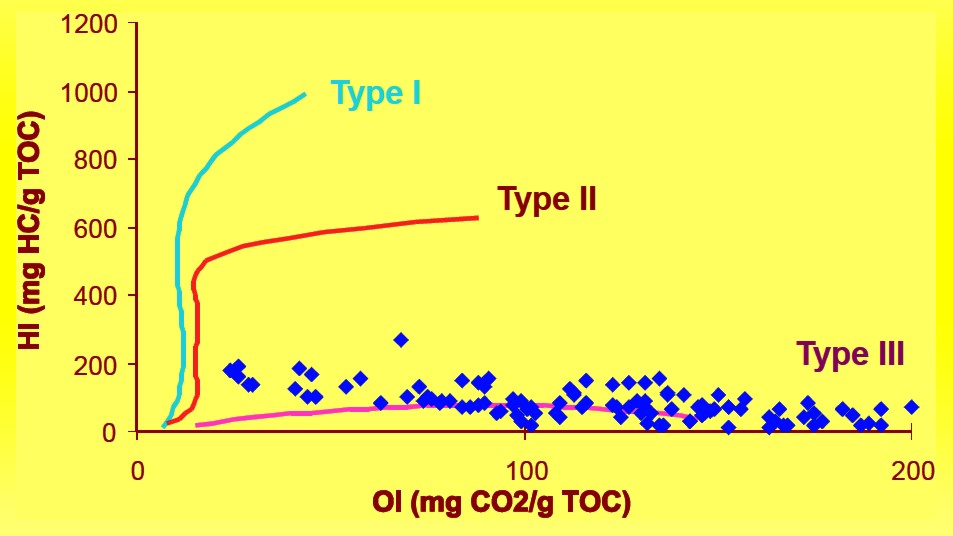
HI versus OI plot example, indicating Type III kerogen
An alternate
method for measuring TOC by solution rather than pyrolysis is
described below, from a 1980's TOC report from Australia.
"The samples are
analyzed for total organic carbon (TOC) according to AS 1038 Part 6.
Moisture determinations are made to permit conversion to a dry
basis. Carbon occurring as carbonate ion is determined to correct
the gross carbon data to give the organic carbon content. This is
done by driving off carbonate minerals with HCl acid.
The crushed and sieved (100 mesh) samples are weighed and
exhaustively extracted in a Soxhlet apparatus using a
benzene-methanol mixture. After removal of methanol by azeotropic
distillation with benzene, the residue in benzene is diluted with
hexane and the hydrocarbon solution separated by filtration from the
brown precipitate. The latter is then dissolved in methanol. The
yield of methanol soluble material is determined gravimetrically.
The hexane soluble portion of the extractable organic matter
(E.O.M.) is weighed and chromatographed on silica. Elution with
hexane gives predominantly alkanes and subsequent elution with
hexane/benzene yields mainly monocyclic and polycycllc aromatic
hydrocarbons. The eluted hydrocarbons are weighed, and then analyzed
by gas chromatography / mass spectrometry."
Geochemical Logs
Measured and calculated indices can be plotted versus depth; the
resulting log
is called a Geochemical Log.
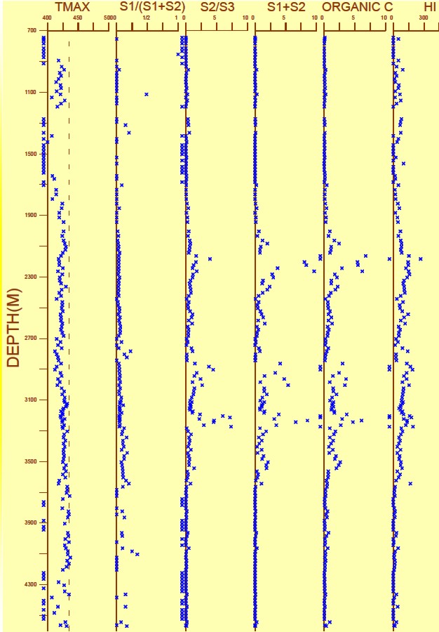
A geochemical log from offshore
East Coast Canada
KEROGEN
maturity
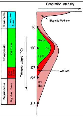 The
hydrocarbon potential of organic carbon depends on the thermal
history of the rocks containing the kerogen. Both temperature and
the time at that temperature determine the outcome. Medium
temperatures
(< 175 C) produce mostly oil and a little gas. Warmer temperatures
produce mostly gas. The
hydrocarbon potential of organic carbon depends on the thermal
history of the rocks containing the kerogen. Both temperature and
the time at that temperature determine the outcome. Medium
temperatures
(< 175 C) produce mostly oil and a little gas. Warmer temperatures
produce mostly gas.
Hydrocarbon
type versus temperature
defines "oil window" and "gas window",
with some obvious overlap
Vitrinite reflectance (Ro) is used as an indicator of the level of
organic maturity (LOM). Ro values between 0.60 and 0.78 usually
represent oil prone intervals. Ro > 0.78 usually indicates gas
prone. High values can suggest "sweet spots" for completing gas
shale wells.
Measurement of vitrinite reflectance was
described as follows from the 1980's TOC report.
"Sample
chips or sidewall core samples are cleaned to remove drilling mud or
mud cake and then crushed using a mortar and pestle to a grain-size
of less than 3 mm. Samples are mounted in cold-setting resin and
polished ''as received", so that whole-rock samples rather than
concentrates of organic matter are examined. This method is
preferred to the use of demineralized concentrates because of the
greater ease of identifying first generation vitrinite and, for
cuttings samples, of recognizing cavings. The core samples are
mounted and sectioned perpendicular to the bedd1ng.
Vitrinite reflectance measurements are made using immersion oil of
refractive index 1.518 at 546 nm and 23°C and spinel and garnet
standards of 0.42%, 0.917% and 1.726% reflectance for calibration.
Fluorescence-mode observations are made on all samples and provide
supplementary evidence concerning organic matter type, and exinite
abundance and maturity. For fluorescence-mode a 3 mm BG-3
excitation filter is used with a TK400 dichroic mirror and a K490
barrier filter."
Tmax is also a useful indicator of
maturity, higher values being more mature.
Graphs of HI vs Ro and HI vs Tmax are
used to help refine kerogen type and to assess maturity with respect
to the oil and gas "windows". Depth plots of Ro and Tmax are helpful
in spotting the top of the oil or gas window in specific wells, and
in locating sweet spots for possible production using horizontal
wells.
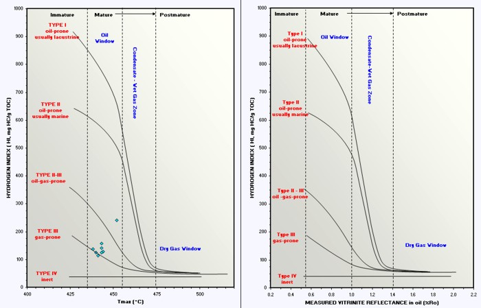
Crossplots of HI vs Tmax and HI vs Ro
determine organic maturity, kerogen type, and whether the rock is in
the oil or gas window. Immature and post mature rocks are not overly
interesting as possible source or reservoir rocks.
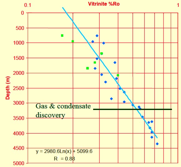
Depth plot of Ro to determine trend line and location of oil and gas
windows (Ro > 0.55).
Ro is plotted on a logarithmic scale, which makes the trend line
relatively straight.
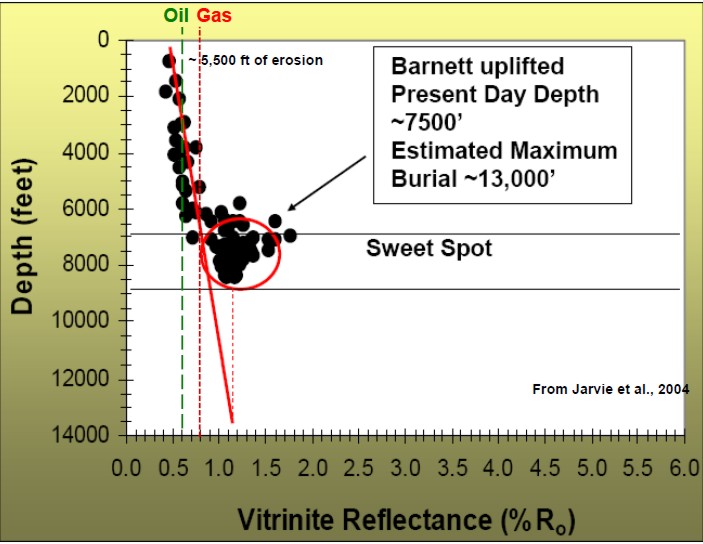
Thermal maturity as indicated by
vitrinite reflectance (Ro) versus depth for a Barnett shale, showing
"sweet spot" and
oil versus gas “windows”.
VISUAL ANALYSIS OF TOC FROM LOGS
 Visual
analysis for organic content is based on the porosity - resistivity
overlay technique, widely used to locate possible hydrocarbon shows
in conventional log analysis. By extending the method to radioactive
zones instead of relatively clean zones, organic rich shales
(potential source rocks , gas shales, oil shales) can be identified.
Usually the sonic log is used as the porosity indicator but the
neutron or density log would work as well. Visual
analysis for organic content is based on the porosity - resistivity
overlay technique, widely used to locate possible hydrocarbon shows
in conventional log analysis. By extending the method to radioactive
zones instead of relatively clean zones, organic rich shales
(potential source rocks , gas shales, oil shales) can be identified.
Usually the sonic log is used as the porosity indicator but the
neutron or density log would work as well.
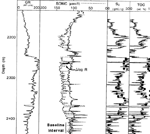
The
trick here is to align the sonic log on top of the logarithmic scale
resistivity log so that the sonic curve lies on top of the
resistivity curve in the low resistivity shales. Low resistivity
shales are considered to be non-source rocks and are unlikely to be
gas shales. Shales or silts with source rock potential will show
considerable crossover between the sonic and resistivity curves.
The absolute value of the sonic and resistivity in the low
resistivity shale are called base-lines, and these base-lines will
vary with depth of burial and geologic age.
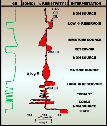
Schematic log showing sonic resistivity overlay in a variety of
situations
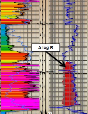
Sonic resistivity overlay showing crossover in Barnett Shale, Texas,
labeled "ΔlogR" and shaded red.
Crossplots of porosity and logarithm of resistivity can also be used
to define and segregate source rocks from non-source rocks. See
"Identification of Source Rocks on Wireline Logs by
Density-Resistivity and Sonic-Resistivity Crossplots" by B. L. Meyer
and M. H. Nederlof, AAPG Bulletin, V. 68, P 121-129, 1984..The
best description of the method is posted on the online magazine
Search and
Discovery,
in
"Direct Method for Determining Organic Shale Potential from Porosity
and Resistivity Logs to Identify Possible Resource Plays* by Thomas
Bowman,
Article #110128, posted June 14, 2010.
These
crossplots usually show a non-source rock trend line on the
southwest edge of the data (similar to the water line on a Pickett
plot) and a cluster of source rock data to the right of the
non-source line, as shown in the image below. The
slope and intercept of the non-source line is used to calculate a
pseudo-sonic log, DtR, from the resistivity log, which can then be
plotted on the same scale as the original sonic log.

Sonic versus logarithm of resistivity (DlogR) Crossplot showing
non-source rock trendline and source rock cluster of data. The
equation of the non-source rock line is DtR = 105 - 25 log(RESD) for
this Barnett Shale example.
 As
for the manual overlay technique described above, crossover
indicates source rock potential, shale gas, or an oil shale, or if
the zone is clean, a potential hydrocarbon pay zone. An example of a
DtR log is shown below. As
for the manual overlay technique described above, crossover
indicates source rock potential, shale gas, or an oil shale, or if
the zone is clean, a potential hydrocarbon pay zone. An example of a
DtR log is shown below.
Original sonic
log (left edge of red shading) and calculated DtR curve (black curve)
showing potential source rock or, as in this case, gas shale (Barnett)
Because porosity indicating logs
suffer from mineralogy, porosity, and shale effects (not to mention
rough and large borehole effects on the density log), as well as the
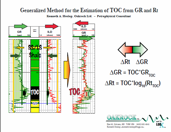
effect of kerogen, Heslop (AAPG 2010) proposed a method of using
gamma ray (GR) and deep Resistivity (RESD) overlays instead of
porosity - resistivity overlays to find intervals with poential for
organic carbon.
In non-source shale (no TOC,), the GR increases while the RESD
decreases, compared to typical reservoir rocks. These two log curves
tend to “hour-glass” when plotted using conventional scales.
Reversing one of the scales causes the GR and RESD curves to track
each other. The exception occurs where TOC is present. When tracking
, the separation gap between GR and RESD should be relatively
constant. When TOC is present, both GR and RESD will increase in
proportion to the TOC, and because of the standard log scales used,
the separation gap increases.
When expressed as the difference between non-source and source roc
log values, the Heslop equation becomes:
1: ΔGR + ΔRESD = TOC * (GRtoc + log(RESDtoc))
Where:
ΔGR and ΔRESD = differences between non-source and possible source rock
values
measured in log grid units
TOC = total organic carbon (mass fraction)
GRtoc and RRESDtoc were determined using TOC lab data correlated to
the GR vs RESD separation gap.
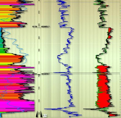
Example from Ken Heslop's AAPG
2010 presentation showung GR and RESD in normal scales in Tracks 1
and 2, with reversed ILD on normal GR in track 3. Moderate separation
gap between these two curves near bottom marked "TOC".
BASIC ANALYSIS OF TOC FROM LOGS
A
wide variety of log analysis methods are used to calculate total
organic carbon from well logs, ranging from over-simplified to
complex multi-mineral probabilistic models. The Passey and Issler
models, described later, are in the middle of the pack for
complexity. We also need to convert lab data into volumetric terms
for comparison to log analyis results. This Section coversd some of
these steps.
IMPORTANT: Remember that all log analysis models for TOC are
calibrated to standard geochemistry lab data that often do not
discriminate between kerogen and pyrobitumen. Either or both may be
present. Both have variable but fortunately similar physical
propertiees so converting log derived TOC to "kerogen" may actually
be a conversion to pyrobitumen or a mixture of the two components.
Correlation of core TOC values to log data leads to useful
relationships for specific reservoirs. A strong correlation exists in some shales with
Uranium content from the spectral gamma ray log. In other cases, the
relationship is made with density, resistivity, sonic, gamma
ray, or combinations of these curves. Variations in matrix
mineralogy strongly affect this type of correlation and it is
possible that mineralogy will mask any trend with TOC. The crossplot
shown below is for a particular well in the Barnett shale.
Correlation of TOC with density in Barnett Shale: Wtoc = -0.259 *
DENS + 0.707. Similar crossplots
of sonic or neutron data can be used for specific reservoirs where
TOC data is available from core.
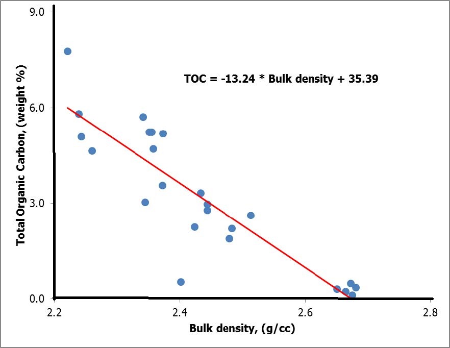
Plot in Avalon Shale: Wtoc = -0.1324 * DENS + 0.754
In their 1983 paper, Schmoker and Hester proposed the
following equation based on data from the very organic rich Upper
and Lower Bakken Shales in North Dakota and Montana:
Wtoc = 0.01 * ((154.49 7 / DENS) – 57.261)
The constants were
specific to these shales and may not apply
elsewhere.Assumptions are based on an organic
matter density of 1.01 g/cc, a matrix density of
2.68 g/cc, and a ratio between weight percent of
organic matter and organic carbon of 1.3. The study
reported an average organic-carbon content
12.1 wt% (upper shale) and 11.5 wt%(lower shale),
using data from more than 250 wells.
It may be
possible to use crossplots other than TOC versus density (DENS).in
local areas. Density may be a poor indicator of TOC due to rough
hole conditions or lithology variations (both clay volume and
mineral mixture variations can add noise to the crossplot).
TOC versus DlogR (or DtR), which was derived in a previous section on this
page, is really a plot of TOC versus deep resistivity (RESD). Both
plots are shown below. Resistivity is not much affected by rough or
large borehole or mineralogy variations, but is affected by water
fraction in porosity and clay volume.
TOC versus uranium (URAN) from a gamma ray spectral log may be
useful. Large variations in boreehole size and variations in the
uranium content of the kerogen may cause noise. If clay volume is
low or nearly constant, the total gamma ray log (GR) may be used. Do
not use the "corrected" gamma ray (CGR) as the uranium has been
removed from that curve. If both GR and CGR are available without
the URAN curve, the difference between GR and CGR is equivalent to
the shape of a URAN curve, so a TOC versus (GR - CGR) may be
useful.
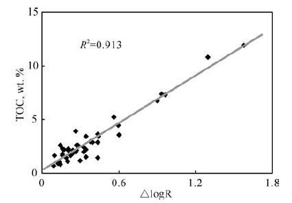
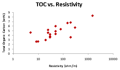

TOC versus DtR
TOC versus log(RESD)
TOC versus URAN
More sophisticated TOC log analysis
models, such as Passey and Issler's methods, are developed later in
ths weboage.
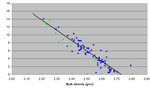
Kerogen Density
Kerogen density is difficult to measure directly but can be inferred
from a plot of (inverse) core grain density versus TOC weight
percent or mass fraction.
This value is needed to find kerogen volume fraction
from kerogen weight fraction. The method also relies on the density
versus TOC crossplot.
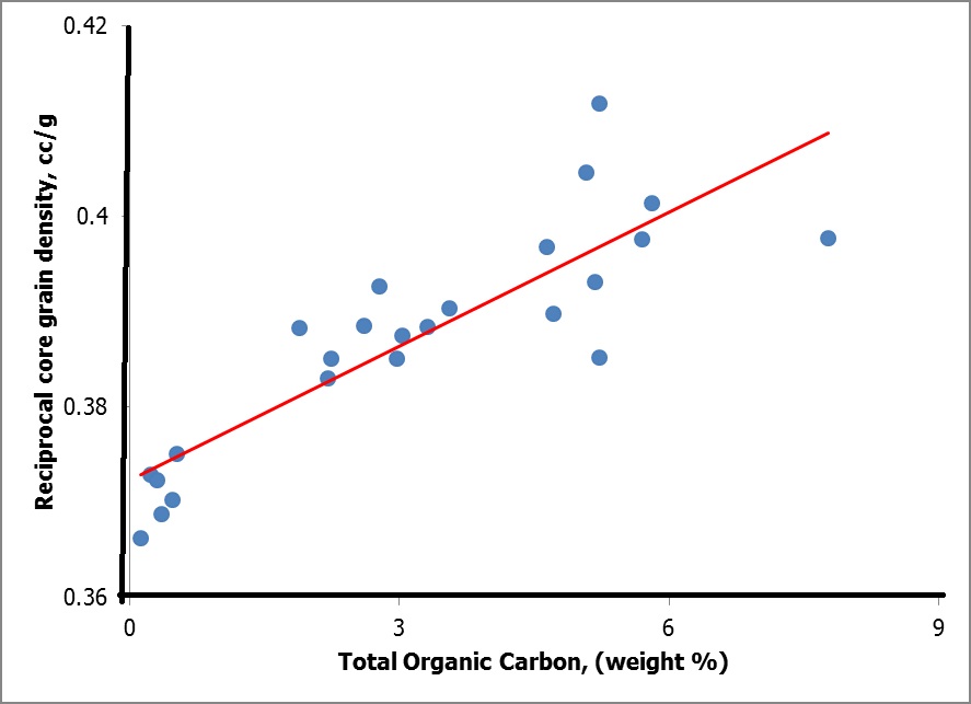
Plot to find TOC specific gravity (DENStoc) and rock grain density (DENSma)
using inverse grain density on Y-Axis.
On
this graph,
1:
DENSma = 1 / INTCPT
= 1 / 0.37 = 2.703 g/cc
2: SLOPE = (0.409 - 0.37) /
(9 - 0) = 0.004166
(from Excel spreadsheet)
3: DENStoc = 1 / (100 * SLOPE + INTCPT)
= 1 / (100 * 0.004166 + 0.37) = 1.28 g/cc
4: DENSker = DENStoc / KTOC
= 1.28 / 0.80 = 1.42 g/cc
Where KTOC = kerogen correction factor
- Range = 0.68 to 0.90, default 0.80
Typical values for DENSker are in the range 0.95 for immature to
1.45 for very mature, with a default of 1.26 g/cc.
Because of the extrapolation from small TOC values up to 100% TOC,
the possible error in DENStoc is quite large, so many people will
choose a default based on the maturity of the kerogen.
Kerogen Volume
Log
analysis models need the volume fraction of kerogen, not the weight
fraction. This is found from:
 1: Wtoc = TOC% / 100
2: Wker = Wtoc / KTOC
3: VOLker = Wker / DENSker
4: VOLmatrix = (1 - Wker) / DENSma
5: VOLrock = VOLker + VOLmatrix
6: Vker = VOLker / VOLrock
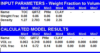
There is
a spreadsheet on the Downloads page
that does weight to volume and volume to weight conversions -- see
example at right.
Typically, Vker is a little less than 2 * Wtoc.
SPR-15 META/LOG WEIGHT <== ==> VOLUME CALCULATOR
Convert weight fraction to / from volume fraction.
GAS CONTENT versus TOC
TOC values calculated from log analysis models
are widely used as a guide to the quality of gas shales. Using
correlations of lab measured TOC and gas content (Gc). We can use log
analysis derived TOC values to predict Gc, which can then be summed
over the interval and converted to adsorbed gas in place. Sample
correlations are shown below.
 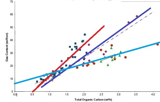
Crossplots of TOC versus Gc for
Tight Gas / Shale Gas examples. Note the large variation in Gc versus
TOC for different rocks, and that the correlations are not always
very strong. These data sets are from core samples, cuttings give
much worse correlations. The fact that some best fit lines do not
pass through the origin suggests systematic errors in measurement or
recovery and preservation techniques.
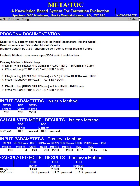
PASSEY'S "DlogR"
METHOD
Various multi-curve methods for quantifying organic content from well logs have
been published, including multiple regression, probabilistic, and
neural network solutions. The most common method is based on sonic versus resistivity,
as described in "A Practical
Model for Organic Richness from Porosity and Resistivity Logs" by Q. R. Passey,
S. Creaney, J. B. Kulla, F. J. Moretti
and J. D. Stroud, AAPG Bulletin, V. 74, P 1777-1794, 1990.
It is also known as the "D log R" method
(with or without spaces and hyphens between the characters). The "D"
was originally the Greek letter Delta (ΔlogR).
Although the sonic resistivity model is the best known version of
the Passey method, density and neutron data can also be used, as
shown below:
1: SlogR = log (RESD / RESDbase) + 0.02 * (DTC –
DTCbase)
2: DlogR = log (RESD / RESDbase) -- 2.5 * (DENS –
DENSbase)
3: NlogR = log (RESD / RESDbase) + 4.0 * (PHIN –
PHINbase)
4: TOCs = SF1s * (SlogR * 10^(0.297 – 0.1688 * LOM))
+ SO1s
5: TOCd = SF1d * (DlogR * 10^(0.297 – 0.1688 * LOM))
+ SO1d
6: TOCn = SF1n * (NlogR * 10^(0.297 – 0.1688 * LOM))
+ SO1n
Where:
RESD = deep resistivity in any zone (ohm-m)
RESDbase = deep resistivity baseline in non-source rock (ohm-m)
DTC = compressional; sonic log reading in any zone (usec/ft)
DTCbase = sonic baseline in non-source rock (usec/ft)
DENS = density log reading in any zone (gm/cc)
DENSbase = density in non-source rock (gm/cc)
PHIN = neutron log reading in any zone (fraction)
PHINbase = neutron baseline in non-source rock (fraction)
SlogR, DlogR, NlogR =
Passey’s
number from sonic, density, neutron log (fractional)
LOM = level of organic maturity (unitless)
TOCs,d,n = total organic carbon from Passey method (weight fraction)
SF1s,d,n and SO1s,d,n = scale factor and scale offset to calibrate to lab values of TOC
Divide metric
DTC values by 3.281 to get usec/ft, metric density by 1000 to get
gm/cc.
In practice, it is rare to have
both TOC laboratory measurements and reliable organic maturity data
to assist in calibration. Chose a value for LOM that will result in
a match with available TOC data.
Vitrinite reflectance (Ro) values may be available and are converted
to LOM with the graph below. LOM is typically in the range of
6 to 14. Default LOM for a gas shale is 8.5 and fir an oil shale
is10.5.
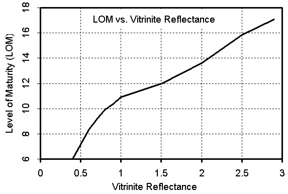
Graph for finding Level of Organic
Maturity from Vitrinite Reflectance. Higher LOM reduces calculated
TOC. Some petrophysicists do not
believe this chart, and use regression techniques on measured TOC to
estimate LOM - see bottom illustration on this page for an example.
Numerical Example:
RESD RESDbase DTC DTCbase LOM DENS DENSbase PHIN PHINbase
25 4 100 62 8.5 2.35 2.65 0.34 0.15
DTC DENS PHIN
DlogR = 1.556 1.546 1.556
TOC = 0.113 0.113 0.113 weight fraction
ISSLER'S METHOD
Dale Issler published a model specifically tuned to Western Canada
in "Organic
Carbon Content Determined from
Well Logs: Examples from Cretaceous Sediments of Western
Canada" by Dale Issler, Kezhen Hu,
John Bloch, and John Katsube, GSC Open File 4362. It is based on density vs resistivity and sonic
vs resistivity crossplots (other methods are also described
in the above paper).
The crossplots were redrafted in
Excel , as shown below, and a drop-through code developed to
generate TOC, based on the lines on the graphs. No doubt
there is a simpler way to code this, but I didn't have time
to sort it out.
 ◄
DTC vs RESD ◄
DTC vs RESD
DENS vs RESD
►
Note that sonic and density data are in Metric
units.
TOC calculated from DENS vs RESD crossplot gives similar
results to the sonic approach, but the density model should
not be used in large or rough borehole intervals. Intervals
where the sonic log is skipping should be edited before use.
The
"drop-through" code shown below gives integer values of
TOC%, then coverts it to a decimal fraction. Multiple
regression equations, developed by Tristan Euzen from the
Issler graphs, give
smooth (non-integer) values and are of course easier to code
into petrophysical software or spreadsheet packages. Thanks
for your work Tristan.
TOC FROM REGRESSION ANALYSIS OF ISSLER'S GRAPHS
Tristan Euzen's multiple regression gives:
7: TOCs =
0.0714 * (DTC + 195 * log(RESD)) - 31.86
8: Wtocs = SF2 * TOCs / 100 + SO2
Equations for the density-resistivity model are not quite as
neat. By linear regression, Tristan found:
97:
Intercept = 4.122 * Slope + 1014
98: TOCd = -0.1429 * Slope + 45.14
Recognizing that:
99: DENS = Slope * Log(RESD) + Intercept
And by substitution:
9: TOCd = -0.1429 * (DENS – 1014) / (log(RESD) + 4.122) + 45.14
10: Wtocd = SF3 * TOCd / 100 + SO3
Log analysis TOC results
should be calibrated to lab measured TOC from real
rocks. Scale factors SF 2 and SF3 and scale offset SO2 and
SO3 are determined by regression of lab versus log derived
TOC values. If you want TOC%, remove the "/ 100" from
equations 8 and 10.
TOC FROM MULTIPLE LINEAR REGRESSION
Sometimes it is difficult to get a good match to measured
TOC values using Passey or Issler methods. Some software
packages have multiple linera equation solvers. that can
help. Here is a typical solution for one particular well
where such a regression was run:
11: TOCmr = - 3.73089 + 0.0259051 * DTC + 1.13726
* PHIN_SS + 0.877866 * log(RESD)
- 0.000722865 * DENS
No scale factor or scale offset is needed as the equation is
derived from the measured data.
TOC from Sonic Resistivity Crossplot
TOC from Sonic Resistivity Crossplot
IF DELT <= (-195 * LOG(RESD) + 460) THEN TOCs = 0
IF DELT > (-195 * LOG(RESD) + 460) THEN TOCs = 1
IF DELT > (-195 * LOG(RESD) + 474) THEN TOCs = 2
IF DELT > (-195 * LOG(RESD) + 488) THEN TOCs = 3
IF DELT > (-195 * LOG(RESD) + 502) THEN TOCs = 4
IF DELT > (-195 * LOG(RESD) + 516) THEN TOCs = 5
IF DELT > (-195 * LOG(RESD) + 530) THEN TOCs = 6
IF DELT > (-195 * LOG(RESD) + 544) THEN TOCs = 7
IF DELT > (-195 * LOG(RESD) + 558) THEN TOCs = 8
IF DELT > (-195 * LOG(RESD) + 572) THEN TOCs = 9
IF DELT > (-195 * LOG(RESD) + 586) THEN TOCs = 10
IF DELT > (-195 * LOG(RESD) + 600) THEN TOCs = 11
IF DELT > (-195 * LOG(RESD) + 614) THEN TOCs = 12
IF DELT > (-195 * LOG(RESD) + 628) THEN TOCs = 13
IF DELT > (-195 * LOG(RESD) + 642) THEN TOCs = 14
IF DELT > (-195 * LOG(RESD) + 656) THEN TOCs = 15
IF DELT > (-195 * LOG(RESD) + 670) THEN TOCs = 16
IF DELT > (-195 * LOG(RESD) + 684) THEN TOCs = 17
IF DELT > (-195 * LOG(RESD) + 698) THEN TOCs = 18
IF DELT > (-195 * LOG(RESD) + 712) THEN TOCs = 19
IF DELT > (-195 * LOG(RESD) + 726) THEN TOCs = 20
IF DELT > (-195 * LOG(RESD) + 740) THEN TOCs = 21
IF DELT > (-195 * LOG(RESD) + 754) THEN TOCs = 22
IF DELT > (-195 * LOG(RESD) + 768) THEN TOCs = 23
IF DELT > (-195 * LOG(RESD) + 782) THEN TOCs = 24
Wtocs = SF2 * TOCs / 100 + SO2
TOC from Density Resistivity Crossplot
IF DENS < (150 * LOG(RESD) + 1670) THEN TOCd = 24
IF DENS < (155 * LOG(RESD) + 1695) THEN TOCd = 23
IF DENS < (160 * LOG(RESD) + 1720) THEN TOCd = 22
IF DENS < (166 * LOG(RESD) + 1745) THEN TOCd = 21
IF DENS < (170 * LOG(RESD) + 1770) THEN TOCd = 20
IF DENS < (176 * LOG(RESD) + 1795) THEN TOCd = 19
IF DENS < (183 * LOG(RESD) + 1820) THEN TOCd = 18
IF DENS < (190 * LOG(RESD) + 1845) THEN TOCd = 17
IF DENS < (197 * LOG(RESD) + 1870) THEN TOCd = 16
IF DENS < (211 * LOG(RESD) + 1895) THEN TOCd = 15
IF DENS < (218 * LOG(RESD) + 1920) THEN TOCd = 14
IF DENS < (225 * LOG(RESD) + 1945) THEN TOCd = 13
IF DENS < (232 * LOG(RESD) + 1970) THEN TOCd = 12
IF DENS < (239 * LOG(RESD) + 1995) THEN TOCd = 11
IF DENS < (246 * LOG(RESD) + 2020) THEN TOCd = 10
IF DENS < (253 * LOG(RESD) + 2050) THEN TOCd = 9
IF DENS < (260 * LOG(RESD) + 2080) THEN TOCd = 8
IF DENS < (267 * LOG(RESD) + 2110) THEN TOCd = 7
IF DENS < (274 * LOG(RESD) + 2140) THEN TOCd = 6
IF DENS < (281 * LOG(RESD) + 2170) THEN TOCd = 5
IF DENS < (288 * LOG(RESD) + 2200) THEN TOCd = 4
IF DENS < (295 * LOG(RESD) + 2232) THEN TOCd = 3
IF DENS < (302 * LOG(RESD) + 2264) THEN TOCd = 2
IF DENS < (309 * LOG(RESD) + 2300) THEN TOCd = 1
IF DENS >= (309 * LOG(RESD) + 2300) THEN TOCd = 0
Wtocd = SF3 * TOCd / 100 + SO3
Log analysis TOC results
should be calibrated to lab measured TOC from real
rocks. Scale factors SF 2 and SF3 and scale offset SO2 and
SO3 are determined by regression of lab versus log derived
TOC values. If you want TOC%, remove the "/ 100" from the
final equations.
Numerical Example
RESD DTC DENS
Using spreadsheet from Downloads page
English 25 100 2.35
Metric 25
328 2350
TOCs (RESD-DTC crossplot) = 0.11 weight fraction
TOCd (RESD-DENS crossplot) = 0.10 weight fraction
META/LOG "TOC" SPREADSHEET
-- TOC ASSAY FROM LOG ANALYSIS
This
spreadsheet calculates Total Organic Carbon (TOC) from the two
different models described above.
SPR-13 META/LOG ORGANIC CARBON (TOD) CALCULATOR
Calculate total organic carbon (TOC), Passey, Issler,
5 Methods
Sample output from META/LOG "TOC" spreadsheet for analysis of Total
Organic Carbon from well logs.
TOC From SpectrAL GAMMA RAY Log
The uranium content of many kerogen bearing source and reservoir
rocks is often a function of the kerogen content. Bob Everett
suggests the following relationship:
1: TOCuran = SFuran * log(URAN / 4)
Where:
TOC uran = total organic carbon from uranium curve on spectral GR loh
(fractional)
URAN = uranium content (ppm)
SFuran = scale factor = 0.05 default (range 0.02 to 0.08)
Calibrate SFuran using lab derived TOC data. Note that the spectral
GR could be a core GR log.
TOC From Elemental Capture Spectroscopy (ECS) Logs
The ECS log measures the weight contribution of various elements in
the formation, for example calcium, oxygen, iron, silicon, and so
forth. By using a least squares statistical approach, the elements
can be composed into the minerals that might be present in the
rocks. One of the minerals can be kerogen. Results are in weight
fraction so kerogen can be compared directly to geochemical assays
from the lab. The TOC and XRD or XRF lab data can be used to
constrain the inversions, giving results that will naturally match
kerogen and mineralogy data quite well. An example is shown at the
end pf this web page.
TOC LOG ANALYSIS EXAMPLES
TOC calculated from Passey DlogR Method. There are numerous
published examples with much worse correlations between calculated
and measured TOC, usually attributed to varying proportions of Type
I, II, and III kerogen or mineral variations (calcite, dolomite,
pyrite, and quartz) in the shale.

The figure above shows a comparison of the DlogR method with the
Issler model. Both methods use sonic and resistivity logs to
calculate the depth variation in TOC. Red dots represent measured
TOC analyzed on core
samples using a Rock-Eval 2 instrument; blue dots represent
re-analyses of the same samples using a Rock-Eval 6 instrument. For
the Issler model, results are presented for both empirical (blue)
and Archie (green) resistivity porosity methods. The DlogR method
gives poor results for this well when observed thermal maturity is
used (LOM = 5.0) An LOM value of 6.9 provides a good fit to the data but
it is not representative of the true maturity.

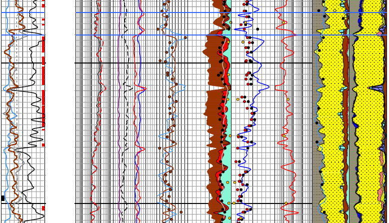
A nuclear magnetic effective porosity curves
(light grey on porosity track) shows a close match to shale and
kerogen corrected density-neutron effective porosity (left edge of red shading).
Dark shading on porosity track is kerogen volume. NMR porosity, and corrected effective porosity
match very well. The NMR effective porosity is unaffected by
kerogen and clay bound water. The far right
hand track is the mineralogy from an Elemental Capture
Spectroscopy (ECS) log in weight fraction (excludes porosity but
includes TOC). TOC from cores, Issler method, and ECS are in the
track to the left of the porosity. They also match quite well.
The ECS inversion was also calibrated to TOC and XRD data to get a match
as good as this. Clay volume in second track from the right is
from thorium curve calibrated to XRD total clay, with clay
volume from ECS superimposed to show the close agreement.
Everything makes sense when you CALIBRATE to lab data but may be
NONSENSE if you don't gather the right data.
|

