IMMATURE OIL Shale BAsics
The immature oil shale case is shown on the rest of this web page. See tight oil plays for the mature kerogen special case.,

The distinguishing characteristic of an immature "oil shale" is that it contains significant organic carbon but no free oil or gas. This hydrocarbon is immature, not yet transformed into oil by natural processes, and are usually termed "source rocks". Some adsorbed and some free gas may also exist. Immature oil shales require a specialized log analysis model because the Archie saturation model is often inappropriate.

Immature oil shale can be mined on the surface or at depth and the rock heated in a retort to convert the organic content to oil. Some valuable by products such as vanadium may also be extracted, but dry clay, ash, and other minerals are a serious waste disposal issue. In-situ extraction using super-heated steam, air, carbon dioxide, or some other heat transfer system is used to convert the organic carbon to oil. Collector wells then extract the oil.

Immature oil shales have been exploited since the mid 1800's. An interesting radio show gives a brief history and an over-hyped future for the Colorado -Utah-Wyoming immature oil shales as seen from the post-war perspective of 1946. Click HERE to listen. You can fast-forward over the first 5 minutes to avoid some really bad scene-setting dialogue. And they "forgot" to mention that Canada was the first to commercially produce kerosene from shale oil in 1846.

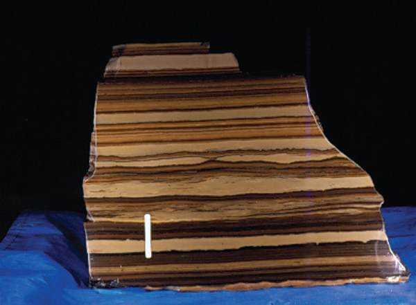
CLASSIFYING OIL Shale
Immature oil shale has received many different names over the years, such as cannel coal, boghead coal, alum shale, stellarite, albertite, kerosene shale, bituminite, gas coal, algal coal, wollongite, schistes bitumineux, torbanite, and kukersite. Some of these names are still used for certain types of oil shale. Recently, however, attempts have been made to systematically classify the many different types of oil shale on the basis of the depositional environment of the deposit, the petrographic character of the organic matter, and the precursor organisms from which the organic matter was derived.

      
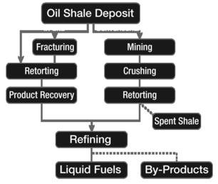
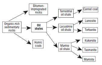
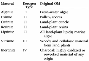
Flowchart for extracting oil from immature oil shale                        Oil shale classification chart                        
 

A useful classification of oil shales was developed by A.C. Hutton. He divided oil shale into three groups based on their deposition environment: terrestrial, lacustrine, and marine, and further by the origin of their organic matter.

Terrestrial oil shales include those composed of lipid-rich organic matter such as resin spores, waxy cuticles, and corky tissue of roots and stems of vascular terrestrial plants commonly found in coal-forming swamps and bogs. Lacustrine oil shales include organic matter derived from algae that lived in fresh, brackish, or saline lakes. Marine oil shales are composed of organic matter derived from marine algae unicellular organisms, and marine dinoflagellates.

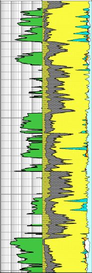
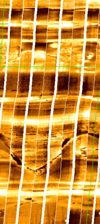Resistivity image log in lacustrine oil shale. White is high resistivity,
black is low resistivity.

Within these three groups, Hutton recognized six specific oil-shale types, as shown in the diagram above:

    1. Cannel coal is brown to black oil shale composed of resins, spores, waxes, and cutinaceous and corky materials derived from terrestrial vascular plants together with varied amounts of vitrinite and inertinite. Cannel coals originate in oxygen-deficient ponds or shallow lakes in peat-forming swamps and bogs.

    2. Lamosite is pale, grayish-brown and dark gray to black oil shale in which the chief organic constituent is lamalginite derived from lacustrine planktonic algae. Other minor components include vitrinite, inertinite, telalginite, and bitumen. The Green River oil-shale deposits in western United States and a number of the Tertiary lacustrine deposits in eastern Queensland, Australia, are lamosites.

    3. Marinite is a gray to dark gray to black oil shale of marine origin in which the chief organic components are lamalginite and bituminite derived chiefly from marine phytoplankton. Marinite may also contain small amounts of bitumen, telalginite, and vitrinite. Marinites are deposited typically in epeiric seas such as on broad shallow marine shelves or inland seas where wave action is restricted and currents are minimal. The Devonian–Mississippian oil shales of eastern United States are typical marinites. Such deposits are generally widespread covering hundreds to thousands of square kilometers, but they are relatively thin, often less than 100 m.
 

    4. Torbanite, named after Torbane Hill in Scotland, is a black oil shale whose organic matter is composed mainly of telalginite found in fresh- to brackish-water lakes. The deposits are commonly small, but can be extremely high grade.

    5. Tasmanite, named from oil-shale deposits in Tasmania, is a brown to black oil shale. The organic matter consists of telalginite derived chiefly from unicellular algae of marine origin and lesser amounts of vitrinite, lamalginite, and inertinite.

    6. Kukersite, which takes its name from Kukruse Manor near the town of Kohtla-Järve, Estonia, is a light brown marine oil shale. Its principal organic component is telalginite derived from green algae. Kukersdite is the main type of oil shale in Estonia and westtern Russiaa, and is burned instead of coal  to generate electricity in power plants.

OIL Shale IN CANADA

Canada produced some shale oil from deposits in New Brunswick in the mid-1800's. The mineral was called Albertite and was originally believed to be a form of coal.

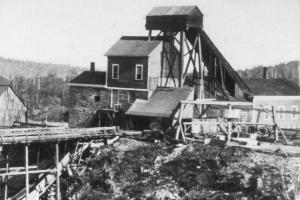
Albert Mines, New Brunswick, in 1850's

Later, the nature of the mineral and its relation to the surrounding oil shale was described correctly. Abraham Gesner used Albertite in his early experiments to distill liquid fuel from coal and solid bitumen. He is credited with the invention of kerosene in 1846, and built a significant commercial distillery to provide lighting oil to replace whale oil in eastern Canada and USA. In the 1880's, shale oil was abandoned as a source of kerosene in favour of distillation from liquid petroleum.

Canada's oil-shale deposits range from Ordovician to Cretaceous age and include deposits of lacustrine and marine origin in at least 20 locations across the country. During the 1980s, a number of the deposits were explored by core drilling. The oil shales of the New Brunswick Albert Formation, lamosites of Mississippian age, have the greatest potential for development. The Albert oil shale averages 100 l/t of shale oil and has potential for recovery of oil and may also be used for co-combustion with coal for electric power generation.

Marinites, including the Devonian Kettle Point Formation and the Ordovician Collingwood Shale of southern Ontario, yield relatively small amounts of shale oil (about 40 l/t), but the yield can be doubled by hydroretorting. The Cretaceous Boyne and Favel marinites form large resources of low-grade oil shale in the Prairie Provinces of Manitoba, Saskatchewan, and Alberta. Upper Cretaceous oil shales on the Anderson Plain and the Mackenzie Delta in the Northwest Territories have been little explored, but may be of future economic interest.
 

Total Organic CARBON (TOC)
Organic content is usually associated with shales or silty shales, and is an indicator of potential hydrocarbon source rocks. High resistivity with some apparent porosity on a log analysis is a good indicator of organic content. Kerogen is the main source of TOC; kerogen is usually radioactive (uranium salts) but the quantity of radioactivity is not a good predictor of the quantity of organic matter..

Oil shales contain predominantly Type I kerogen, as opposed to coal and coal bed methane reservoirs, which contain mostly Type III. Gas shales contain mainly Type II kerogen.

Various methods for quantifying organic content from well logs have been published. The most useful approaches are based on density vs resistivity and sonic vs resistivity crossplots. Other approaches using core measured TOC versus log data, for example density or sonic readings are also common. See TOC Calculation for details.

Determining OIL YIELD (Grade) of Oil Shale FROM ROCK SAMPLES
The grade of oil shale has been determined by many different methods with the results expressed in a variety of units. The heating value of the oil shale may be determined using a calorimeter. Values obtained by this method are reported in English or metric units, such as British thermal units (Btu) per pound of oil shale, calories per gram (cal/gm) of rock, kilocalories per kilogram (kcal/kg) of rock, megajoules per kilogram (MJ/kg) of rock, and other units.

The heating value is useful for determining the quality of an oil shale that is burned directly in a power plant to produce electricity. Although the heating value of a given oil shale is a useful and fundamental property of the rock, it does not provide information on the amounts of shale oil or combustible gas that would be yielded by retorting (destructive distillation).

The grade of oil shale can be determined by measuring the yield of oil of a shale sample in a laboratory retort. The method commonly used in Canada and United States is called the modified Fischer assay, first developed in Germany, then adapted by the U.S. Bureau of Mines. The technique was subsequently standardized as the ASTM Method D-3904-80. Some laboratories have further modified the Fischer assay method to better evaluate different types of oil shale and different methods of oil-shale processing.

The standardized Fischer assay consists of heating a 100-gram sample crushed to –8 mesh (2.38-mm mesh) screen in a small aluminum retort to 500ºC at a rate of 12ºC per minute and held at that temperature for 40 minutes. The distilled vapors of oil, gas, and water are passed through a condenser cooled with ice water into a graduated centrifuge tube. The oil and water are then separated by centrifuging. The quantities reported are the weight percent of shale oil, water, shale residue, and “gas plus loss” by difference. Some organic matter is turned to char and reported as part of the shale residue. As a result, this assay may understate the amount of oil that might be recovered in a commercial scale retort that continuously mixes the feedstock. Oil yield is usually converted from mass fraction into US or Imperial gallons per ton (gpt or gal/t) of rock. So much for going metric! In Canada, oil yields are quoted in liters per metric ton of rock (l/t).
 

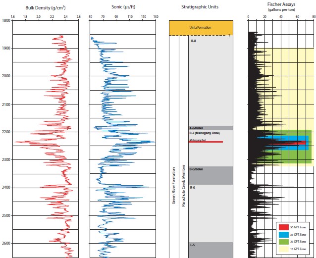
Oil shale example from Utah; density log (left), sonic (middle, Fischer oil yield in gallons/ton (right). Note sonic scale is reverse of conventional oilfield practice. Low density and high sonic travel time correspond to high oil yield, analogous to high porosity in conventional oilfield applications.
 

Determining OIL YIELD (Grade) of Oil Shale FROM WELL LOGS
Traditional methods for log analysis of oil shales, dating back to the early 1960's,  are somewhat over-simplified regression methods using sonic or density data. See for example "Evaluating Oil Shales by Well Logs" by S. R. Bardsley and S. T. Aigermissen, AIME, 1962.

By crossplotting Fischer assay oil yields with corresponding log data, regression lines are generated that provide a decent average oil yield from logs. Problems related to matrix density or matrix travel time variations due to mineral variations with depth are masked by this method. Separate transforms are usually taken when mineralogy is known to change. Logs average about 3 feet (1 meter) of rock compared to much finer detail available from the core assay, so crossplots tend to show considerable scatter in laminated intervals, as shown in the examples below..

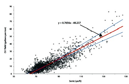Sonic log data versus oil yield from Utah example. Reduced major axis best fit is the most appropriate regression method (red line). Y-on-X and X-on-Y regression lines are also shown. Sonic is in usec/foot, oil yield is in US gallons/ton (gpt or g/t)of rock.

Equation of the line is:
  1: Y = 0.766 * DTC - 49.4
 

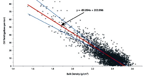
Density versus oil yield for same data set. Density
is in grams/cc

Equation of the line is:
  2: Y = - 80.3 * DENS - 204

Data is from "Basin-Wide Evaluation of Uppermost Green River Oil Shale Resources, Uinta Basin, Utah and Colorado" by M. D. Vanden Berg, Utah Geol Survey, 2008.

Equations for each individual well were also presented, showing considerable variation from well to well and zone to zone.

 
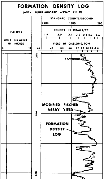
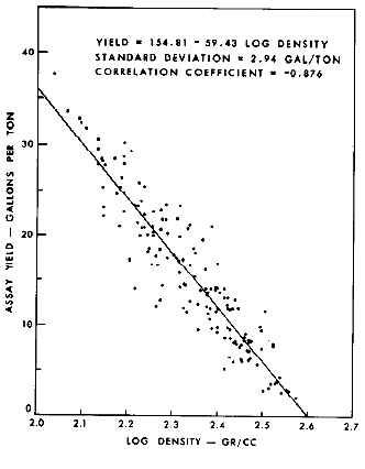
Portuib of debsity log with Fischer core assay (dashed line) and crossplat of density and oil yield, from "Log Evaluation of
Non-Metallic Minerals" SWSC, by M,P, Tixier and R.P/ Alger

A literature search quoted by R. M. Habiger and R. H. Robinson in 1985 gives the following equations for estimating oil yield:
  Smith (1956) Garfield County, Colorado:
      3: Y = 31.6 * DENS^2 - 206 * DENS + 327
      4: Y = 22.9 * DENS^2 - 167 * DENS + 280

  Bardsley and Algermissen (1963) Unita Basin, Utah:
      5: Y = - 66.4 * DENS + 171
      6: Y = 41.01x10^-4 = DTC^2 - 16.7

  Tixier and Alger (1967) Piceance Basin, Colorado:
      7: Y = - 59.4 * DENS + 155

  Cleveland-Cliffs (1975) Uinta Basin, Utah
      8: Y = 496 * DENS^-0.6 - 285
      9: Y = 157 * 10^-4 * DTC^1.8 - 39.2

I have reduced all equations to 3 significant digits, which is all that log analysis can support. The reader should refer to the appropriate technical papers to see the data spread and regional environment before using any of the above equations.

NUMERICAL EXAMPLE
  DENS	2.2	1.8  g/cc
  DTC	100	130  usec/ft
Smith
  3:	26.7	58.6   US gal/ton
  4:	23.4	53.6
					

Bardsley and Algermissen
  5:	24.9	51.5
  6:           24.3	52.6
	

Tixier and Alger
  7: 	24.3	48.1

Cleveland-Cliffs
  8:	24.0	63.6
  9: - 	23.3	61.0

MULTIPLE REGRESSION (PHILLIPS) METHOD
A more sophisticated method was proposed by R. M. Habiger and R. H. Robinson in 1985, using multiple linear regression of sonic, density, and resistivity versus oil yield. The method was patented by the authors on behalf of Phillips Petroleum (US Patent #4548071), even though the method is strictly mathematical and no "invention" was involved. The patent actually claims to protect every individual step of the math, including taking the logarithm of resistivity. Since mathematical solutions and computer code cannot be patented, infringement is moot. Both sonic and density crossplots of the type shown above are included in the patent and in their 1985 SPWLA paper.

They were also faced with very poor quality density log data from poorly calibrated slim hole, non-contact tools. As a result, they had to normalize the density logs using histograms and correlated density "variation" (DV) to oil yield instead of raw density. DV was calculated from:
      10: DV = DENSlog - DENSmean

This also had the effect of handling some of the matrix density variations between wells, but not from layer to layer within each interval in a single well.

A clay index was generated by regression:
      11: CI = DTC + 127.31 * DV - 84.84

Their regression line is quoted as:
   Upper zone:
      12: Y = - 74.37 * DV + 7.86 * (log  RESD) + 0.5 * CI - 9.65
   Lower Zone
      13: Y = - 81.58 * DV + 4.70 * (log RESD) + 9.36

Where"
  DENSlog = actual log reading (gm/cc)
  DENSmean = average density log readings over the analyzed interval (gm/cc)
  DV = density variation (gm/cc)
  DTC = compressional sonic travel time (usec/ft)
  CI = clay  index (percent)
  RESD = deep resistivity reading (ohm-m)
  Y = oil yield (gallons per ton of rock).

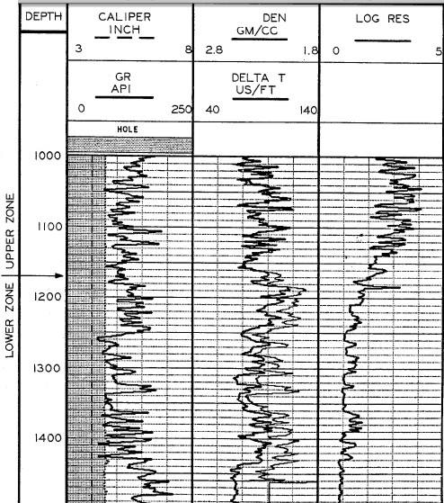
This is the log data from the paper and patent application. Unfortunately neither
document contains an answer plot or Fischer assay data plotted versus depth. Note that
both density and sonic scales are reversed compared to normal oilfield practice.

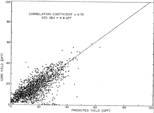
Comparison of Fischer assay oil yield versus yield predicted from multiple regression.

Multi-mineral models for IMMATURE OIL SHALE  evaluation
There are no good reasons to avoid standard multi-mineral methods such as simultaneous equations, principal components, or other statistical methods for oil shales. Simultaneous equation solutions are widely used in mineral evaluation from logs and are covered elsewhere in this Handbook. A typical equation set for an oil shale would be:
    14: DENS = 2.35 * Vshl + 2.65 * Vqtz + 2.74 * Vlim + 2.87 * Vdol + 0.95 * Vker
    15: DTC   = 120 * Vshl + 55 * Vqtz + 47 * Vlim + 44 * Vdol + 200 * Vker
    16: PHIN = 0.30 * Vshl - 0.05 * Vqtz + 0.00 * Vlim + 0.04 * Vdol + 0.95 * Vker
    17: PE  = 3.45 * Vshl + 1.85 * Vqtz + 5.10 * Vlim + 3.10 * Vdol + 0.95 * Vker
    18: 1.00 = Vshl + Vqtz + Vlim + Vdol + Vker

This equation set is inverted by Cramer's Rule or with spreadsheet functions to obtain the unknown volumes. Parameters must be adjusted to suit local conditions. Minerals chosen must be guided by local knowledge, based on petrography or XRD results. If a log curve is unavailable or faulty due to bad hole conditions, the data can be synthesized or the equation set reduced to eliminate that curve, with the loss of one of the minerals in the answer set.

The volumetric results must then be converted to mass fraction, as is done for tar sands, potash, and coal analysis:
      19: WTshl = Vshl * 2.35
      20: WTqtz = Vqtz * 2.65
      21: WTlim = Vlim * 2.71
      22: WTdol = Vdol * 2.87
      23: WTker = Vker * 0.95
      24: WTrock = = WTshl + WTqtz + WTlms + WTdol + WTker

Mass fraction
      25: Wker = WTker / WTrock
      26: WT%ker = 100 * Wker

Where:
  Vxxx = volume fraction of components
  WTxxx = weight of components
  Wxxx = mass fraction of components
  WT%xxx =  weight percent of components

Density parameters must match those used in the original simultaneous equation set.

Kerogen mass fraction should be close to Oil Yield mass fraction from Fischer analysis, or a simple linear conversion to account for "gas plus loss". If Fischer analysis is given in US gal / ton or liters / ton, suitable conversion factors must be used to obtain mass fraction (ton / ton) for comparison to the log analysis results.

Calibration to Fischer assay data would permit adjustment of parameters to produce a better match to core than is usual from single or multiple regression. The core data should be averaged over a 3 foot running average so that comparison to logs can be more meaningful.

I have had no chance to test simultaneous or PCA approach on oil shale, but have used it successfully in potash and conventional multi-mineral oil reservoirs.

META/LOG "YIELD" SPREADSHEET -- IMMATURE OIL SHALE ASSAY FROM LOG ANALYSIS
This spreadsheet calculates an Oil Shale Assay that can be used to evaluate oil shale quality and provides a comparison with Fischer core analysis data.

SPR-17 META/-LOG SHALE OIL YIELD CALCULATOR
  Calculate oil yield in immature oil shale, 6 methods.
 

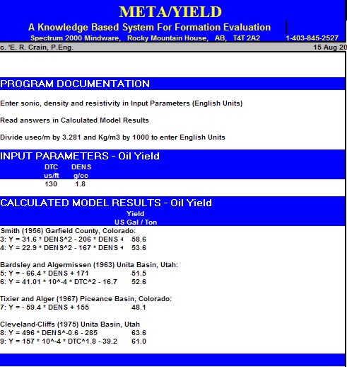
Sample output from "META/YIELD" spreadsheet for oil shale qusality analysis.
 

OIL SHALE EXAMPLE

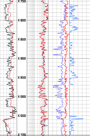
Raw data and computed results in an oil shale. Calculated oil yield is in 2nd track from the right on a logarithmic scale of 1000 to 1.0 US gal/ton.