Modeling the Sonic and Density Response From Regression
Jay Patchett proposed a sonic editing technique in 1975 for shales, based on the following:
      1: log(COND) = A0 + A1 * log(DTC - 42)
            + A2 * log(CEC) + A3 * log(ES)

Where:
  CEC = cation exchange capacity of the shale
  ES = effective stress (psi)

Since CEC is not readily available in most wells, this approach was not terribly practical. However, by recognizing other work that related CEC to gamma ray log response, the equation becomes:

For shale zones:
      2: log(DTDsyn - 40) = KW0 + KW1 * log(RSH)
              + KW2 * log(GR) + KW3 * log(ES)

A similar equation for density is:
      3: DENSsyn = KX0 + KX1 * GR + KX2 * DEPTH + KX3 * log (RSH)

For sandstones:
      4: DTCsyn = KY0 + KY1 * GR + KY2 * log(ES) + KY3 * PHIrs
      5: DENSsyn = KZ0 + KZ1 * GR + KZ2 * DEPTH + KZ3 * PHIrs

Where:
  PHIrs = porosity from the shallow resistivity log

These models are decidedly not simple and a great deal of calibration is required to make them work. Practitioners should refer to the original paper for details of the method. In addition, a sophisticated multiple linear regression program is required.

Case History - Multiple Regression Editing
Here are three US examples from Patchett's work showing:
   1. effect of sonic edits on synthetic
   2. creation of synthetic sonic and density, with resulting synthetic seismogram
   3. comparison of regression derived synthetic with real data

Log editing by multiple regression - original and edited logs and seismogram trace

Synthetic sonic and density log from multiple regression

Comparison of synthetic to real seismic section

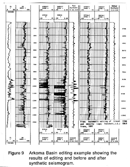
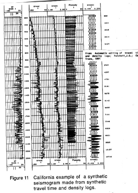
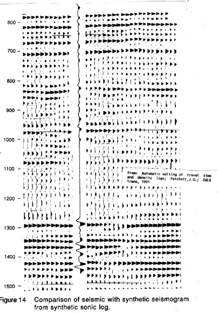
Other examples are contained in the original paper and are well worth reviewing. See "Automatic editing of travel time and density logs", Patchett,J.G.; CWLS Trans, 1991.