Biot's original paper in 1956 pointed out that sonic velocity varied with frequency and described a low frequency case (typically 5 to 35 KHz under normal reservoir conditions) and high frequency case (typically 100 KHz to 1 MHx). Logging tools usually operate in the low frequency range and conform to Biot's low frequency case except in high porosity (> 35%). Sonic velocity measurements made under laboratory conditions are usually made at 1 MHz because the core plugs are small and the high frequency has a short enough wavelength to fully penetrate the sample. R. A. Anderson's paper in 1984 gave graphs of both high and low frequency data versus Wyllie porosity. By comparing
the response of the two frequencies, we can create equations to
convert high frequency data to equivalent low frequency (logging
tool) values. Travel times taken at high frequency are too fast
(DTShi is too low). Where:
Use ONLY to convert lab measured high frequency (1 MHz) sonic data to equivalent low frequency sonic log or seismic frequency data.
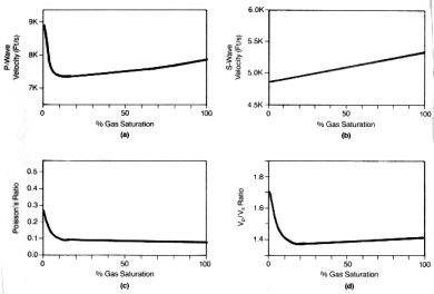
The plots below shows the effect of gas on compressional and shear velocity for a typical rock sample at 6000 feet with 30 percent porosity, calculated from the Biot equations. Notice that compressional velocity drops rapidly with very small gas saturations, compared to the water filled case. Shear velocity increases very slightly with gas and is therefore little affected. Poisson's Ratio and velocity ratio Vp/Vs also decrease with small gas saturations and then remain roughly constant regardless of saturation.
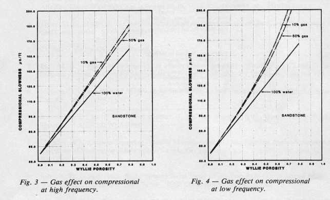
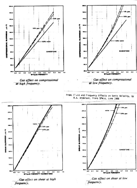
The gas effect on compressional and shear travel time are given below as a function of porosity. These charts can be used to estimate DELTmod for most clean gas bearing rocks. These results underestimate the gas effect when compared to the pseudo-travel time method, but are probably more realistic in shallow to medium depths (3000 to 8000 feet). The effect at low (seismic wavelet) frequency is much stronger than it is for high (sonic log) frequencies.
In
the range of 5 to 30% porosity, all the lines can be
approximated by straight lines. By comparing the gas saturated
lines with the water saturated lines for the low frequency data, we obtain: DTCmodwtr and DTSmodwtr are the compressional and shear travel times for a water-filled reservoir. In water zones, these values could be the actual log readings if there are no obvious borehole effects. In gas zones, where the sonic log sees some residual gas, the values are obtained from the response equation described earlier, using log analysis results for porosity and lithology, and SW = 1.00. The effect on the ratio of shear to compressional travel time (Vp/Vs Ratio) is shown below. The effect at low (seismic wavelet) frequency is much stronger than it is for high (sonic log) frequencies. Therefore, the low frequency data should be used in modeling sonic log response so that it will match the seismic impulse response.
There is no shortage of alternative fluid replacement methods
published since our original work in 1979 and Anderson's in 1984: Castagna, Greenberg
and Castagna, Aki and Richards, Batzie and Wang, Toksoz et al,
Krist,
among others. Use caution when applying these alternate models;
for example Toksoz gets opposite results to Anderson when
computing gas bearing zones. Obviously, some parameters or
assumptions must be different. |
|
||||||||||||||||||||||||||||||||||||||
|
Page Views ---- Since 01 Jan 2015
Copyright 2023 by Accessible Petrophysics Ltd. CPH Logo, "CPH", "CPH Gold Member", "CPH Platinum Member", "Crain's Rules", "Meta/Log", "Computer-Ready-Math", "Petro/Fusion Scripts" are Trademarks of the Author |
|||||||||||||||||||||||||||||||||||||||

|
||
| Site Navigation | LOG EDITING FREQUENCY and GAS EFFECTS ON ACOUSTIC WAVES | Quick Links |