a petrophysical analysis, or the elastic properties of the rocks. Rough borehole conditions and gas effect are the most common problems that will need to be repaired. Exactly what you do to reconstruct the log data will depend on what you want to do with that data. For example, in a conventional quantitative petrophysical analysis, we go to great lengths to avoid using bad data to obtain our results. Gas effect in the invaded zone is handled by well established mathematical techniques or by calibration of results to core analysis data if the logs are inadequate for the purpose. For stimulation design modeling, you want the logs to accurately represent a water-filled reservoir. Since logs read the invaded zone, light hydrocarbons (light oil or gas) make the density log read too low and the sonic log read too high, compared to the water filled case. The magnitude of the error cannot be estimated without reconstructing the logs from an accurate petrophysical analysis. The light hydrocarbon effect problem alone would lead to erroneous elastic properties and erroneous Poisson' Ratio, Young's Modulus, and closure stress predictions. Add some rough borehole effects, and you have a meaningless set of elastic properties for stimulation modeling. Don't despair, there is a solution. Geophysicists modeling seismic response also need good log data for creating synthetic seismograms, calibrating seismic inversion models, and for direct hydrocarbon detection models. The problem here is quite different than either the petrophysical analysis or stimulation design cases. If light hydrocarbon effect exists in the invaded zone, this must be removed and then replaced by a set of log values representing the un-invaded reservoir condition. This is the opposite of the stimulation design problem. In seismic modeling in light hydrocarbons, the density does not read low enough and the sonic does not read high enough to represent the undisturbed reservoir. Unless we fix this, reflection coefficients are too small, inversion models of Poisson's Ratio will not be calibrated, and direct hydrocarbon interpretations will be misleading. We call this process log editing, or log repair, or log reconstruction, or log modeling . We can also create missing log curves by the same reconstruction methods. Some calibration data is required from offset wells to do this reliably. The reconstructed logs are often called synthetic logs, to distinguish them from the original measured data set.
Reconstruction techniques are not new - they have been with us since
the beginning of computer aided log analysis in the early 1970's.
The problem is that few people understand the need for the work or
are unfamiliar with the appropriate techniques.
The workflow for log reconstruction requires a competent petrophysical analysis for shale volume, porosity, water saturation, and lithology using as little bad log data as possible. These results are then "reverse engineered" to calculate what the log "should have read" under the modeled conditions we have imposed. The parameters required will vary depending on whether the reconstruction is for a water-filled case, an invaded-zone case, or an undisturbed reservoir, but the mathematical model is identical for all three cases.
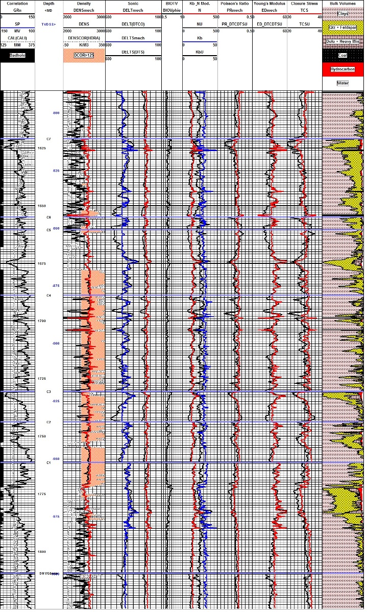
Example of synthetic density and sonic logs used to calculate
elastic properties for a fracture design study. Track 1 has GR,
caliper, and bad hole flag (black bar). Track 2 has density
correction (dotted curve), neutron (dashed), original density (red),
synthetic density (black). Track 3 shows the synthetic
shear, and original and synthetic compressional sonic log curves. In this well, the sonic
did not need much improvement - only small spikes were removed by
the log modeling process. There are a dozen published methods for generating synthetic logs, some dating back more than 60 years, long before the computer era. Most are too simple to do a good job, others are too complicated to be practical. The most successful and practical model to implement and manipulate is the Log Response Equation. This equation represents the response of any single log curve to shale volume, porosity, water saturation, hydrocarbon type, and lithology. Log editing and creation of synthetic logs is absolutely necessary in rough boreholes or when log curves are missing. Fracture design based on bad data guarantees bad design results. Seismic
modeling, synthetic seismograms, and seismic inversion
interpretations are worthless if based on bad log data.
The equations needed are:
3:
KS8 = SUM (Vxxx * (DTS?DTCmultiplier)) Where:
Equation 1 is physically rigorous. Equation 2 is the Wyllie time-average equation, which has proven exceedingly robust despite its lack of rigor. Numerical constants in Equation 3 may need some Sharp eyed readers will notice
that there is a porosity term in Equation 2, which means that
Equation 4 also depends on porosity. Everyone knows that a fluid in
a pore does not support a shear wave, but porosity does affect shear
wave travel time in a manner similar to the compressional travel
time. Consider the following equations: Bulk moduli are in GPa, density is in kg/m3, and sonic travel times are in usec/m in these equations. It is clear from Equations 6 and 7 that both DTC and DTS depend on density, which in turn depends on mineral composition, porosity, and the type of fluid in the porosity. Both Kc and N depend on mineral composition and the presence of porosity. Parameters used in the response equations are chosen appropriately for the case to be modeled. The Sw term varies with what you are trying to model. If you want to model the undisturbed state of the reservoir, Sw is the water saturation from a deep resistivity log and an appropriate water saturation equation. If you want to see what a log would actually read in that zone, you need the invaded zone water saturation, because that's what most logs see. Invaded zone saturation, Sxo, can be derived using a shallow resistivity curve, or it can be assumed to be Sw^(1/5). If you want to see what a water zone would look like, Sw is set to 1.00. That is what we do for a reconstruction destined to be used in calculating rock mechanical properties for stimulation design. In all cases, you need to select fluid parameters to match the assumptions of the model. For example, to reconstruct a log run through an invaded gas zone to reflect the undisturbed case, you need to use the undisturbed zone water saturation and appropriate fluid properties for the water and gas in each equation. Note that for stimulation design, a gas model is not required. For seismic modeling, it is required. Matrix and fluid values for each required log curve are given in Table 1. They may need some tuning to obtain a good match to measured values. Shale values are chosen by observation of the log readings in shale intervals. You may have to look to offset wells to find a shale that does not suffer from bad hole effects.
Density of gas at reservoir conditions The
straight line on the graph is:
The hydrocarbon "pseudo-travel-time" is derived empirically by comparing results from synthetic seismograms and properly processed field data. A very rough approximation of hydrocarbon "pseudo-travel-time" with depth, which has given reasonable results in the western Canadian rock sequences, is shown at left. Travel time for liquids, such as oil and salt water (formation water) are more predictable and may be used in the Wyllie equation without reservation.
This approach was first introduced by the author and John Boyd and published as "Determination of Seismic Response Using Edited Well Log Data" by E.R. Crain and J.D. Boyd at CSEG Annual Symposium, October 1979. The
straight line portion of this graph is represented by: For
oil, we have used: Where: For shear travel time, the porosity can be accounted for by using:
Tune these parameters by comparing the synthetic shear sonic with measured shear data in an offset well.
In
the absence of a full petrophysical analysis, the
following equations will also provide better data than the raw
log data. In gas zones only: Where:
|
|
|||||||||||||||||||||||||||||||||||||||||||||||||||||||||||||||||||||||||||||||||||||||||||||||||||||||||||||||||||||||
|
Page Views ---- Since 01 Jan 2015
Copyright 2023 by Accessible Petrophysics Ltd. CPH Logo, "CPH", "CPH Gold Member", "CPH Platinum Member", "Crain's Rules", "Meta/Log", "Computer-Ready-Math", "Petro/Fusion Scripts" are Trademarks of the Author |
||||||||||||||||||||||||||||||||||||||||||||||||||||||||||||||||||||||||||||||||||||||||||||||||||||||||||||||||||||||||

|
||
| Site Navigation | ROCK PHYSICS EDITING LOGS WITH THE LOG RESPONSE EQUATION | Quick Links |
 In
intervals where there is no bad hole or light hydrocarbon, the
reconstructed logs should match the original log curves. If it
does not, some parameters in the petrophysical analysis or the
reconstruction model are wrong and need to be fixed. It may take a
couple of iterations. Remaining differences are then attributed to
the repair of bad hole effects and light hydrocarbons in the invaded
zone. It is clear from this that the reconstruction needs to
encompass somewhat more than the immediate zone of interest, but not
the entire borehole.
In
intervals where there is no bad hole or light hydrocarbon, the
reconstructed logs should match the original log curves. If it
does not, some parameters in the petrophysical analysis or the
reconstruction model are wrong and need to be fixed. It may take a
couple of iterations. Remaining differences are then attributed to
the repair of bad hole effects and light hydrocarbons in the invaded
zone. It is clear from this that the reconstruction needs to
encompass somewhat more than the immediate zone of interest, but not
the entire borehole. NOTE:
Stimulation design software wants the water filled case for its
input parameters. To accomplish this, set Sw = 1.00 in equations 1
and 2, DENShy and DTChy are therefore not needed.
NOTE:
Stimulation design software wants the water filled case for its
input parameters. To accomplish this, set Sw = 1.00 in equations 1
and 2, DENShy and DTChy are therefore not needed. 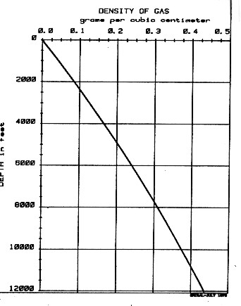 The
DENSsyn
equation is rigorous and can be used with real hydrocarbon densities
based on the temperature, pressure, and phase relationship of the
fluid in question. A chart showing approximate gas density versus
depth is shown at the right, based on average pressure and
temperature data for the western Canadian basin.
The
DENSsyn
equation is rigorous and can be used with real hydrocarbon densities
based on the temperature, pressure, and phase relationship of the
fluid in question. A chart showing approximate gas density versus
depth is shown at the right, based on average pressure and
temperature data for the western Canadian basin. 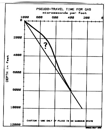 Laboratory
experiments and theory have shown that the time average relationship is
usually not true when gas fills the pore space, or is even a
small fraction of the pore space. For this reason, we call the
hydrocarbon travel time in the Wyllie equation a
"pseudo-travel-time" to reaffirm that it represents a velocity
which may not be the same as the velocity of the gas at the
temperature and pressure of the formation.
Laboratory
experiments and theory have shown that the time average relationship is
usually not true when gas fills the pore space, or is even a
small fraction of the pore space. For this reason, we call the
hydrocarbon travel time in the Wyllie equation a
"pseudo-travel-time" to reaffirm that it represents a velocity
which may not be the same as the velocity of the gas at the
temperature and pressure of the formation.