Calculating Overburden Pressure
Overburden pressure is caused by the weight of the rocks above the formation pressing down on the rocks below. This is sometimes called overburden stress - stress and pressure have the same units of measurement.

Integrating the density log versus depth or estimating the average rock density profile and integrating will calculate this pressure:
      1. Po = KS9 * SUM (DENSi * INCR)

Where:
  Po = overburden pressure (KPa or psi)
  DENSi = density log reading at the i-th data point (kg/m3 or gm/cc)
  INCR = digital data increment (meters or feet)
  KS9 = 0.01 for metric units
  KS9 = 0.0605 for English units

Overburden pressure gradient is:
      2: (Po/D) = Po / DEPTH

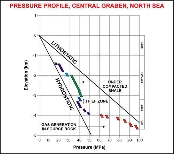
A literature search will turn up some relationships for (PO/D) for specific areas, such as this one for the North Sea:
      3: (Po/D) = (ln(DEPTH - EKB) - 0.5185) / 3.47

In this equation, depth is in meters.
NOTE: All depths must be true vertical depths.

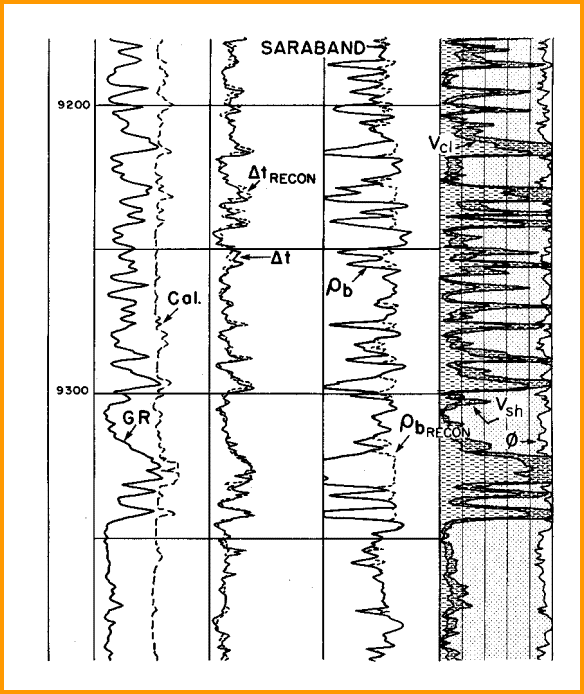
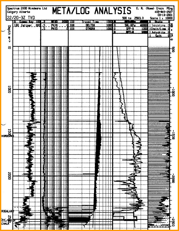
For a real rock sequence, these values may be integrated over each lithologic interval, or can be used to replace density log data over bad hole or missing log intervals. If the density log is in porosity units, use the appropriate transforms to build a density log. The log below shows the type of editing that might be needed on a density log before integration.

Editing density logs based on the log response equation applied to a competent petrophysical
analysis of valid data.

Calculating Normal Pore Pressure
Normal pore pressures occur in many parts of the world. Normal pressure gradients depend only on the density of the fluid in the pores, integrated from surface to the depth of interest. Fresh water with zero salinity will generate a pressure gradient of 0.433 psi/foot or 9.81 KPa/meter. Saturated salt water generates a gradient of 0.460 psi/ft or 10.4 KPa/meter.
      4: Pp = KP1 * DEPTH
      5: Ps = KP2

Formation pore pressure gradient is:
      6: (Pp/D) = Pp / DEPTH

Where:
  DEPTH = formation depth (ft or meters)
  Pp = formation pressure (psi or KPa)
  (Pp/D) = formation pressure gradient (psi/ft or KPa/meter)
  Ps = surface pressure (psi or KPa)
  KP1 = 0.433 to 0.460 psi/foot for English units
  KP1 = 9.81 to 10.4 KPa/meter for Metric units
  KP2 = 14.7 psi for English units
  KP2 = 101 KPa for Metric units

NOTE: All depths must be true vertical depths.

Formation pore pressure (Pp) is the pore pressure used fracture pressure equations. The best source of pore pressure data is the drill stem test (DST) or repeat formation tester (RFT) extrapolated formation pressures from many zones in many wells, plotted versus depth. Commercial databases containing this information are available, or the data can be tabulated from well history files.

The slope (Pp/D) of a series of best fit straight lines drawn through the data points will provide the pressure gradient required. The hydrocarbon content will give lower gradients: oil gives a Pp/D between 0.30 and 0.43 psi/ft (6.78 to 9.81 KPa/m). Gas zones will have gradients from 0.05 to 0.30 psi/ft (2.26 to 6.78 KPa/m). Partially depleted reservoirs may have abnormally low pore pressure if there is no active aquifer, water injection, or gas injection to support the reservoir pressure.

Pore pressure plot versus depth for North Sea - straight line at left is normal pore pressure, line at right is overburden pressure, dots are measured pore pressure.

Some engineering problems require the initial formation pressure, before any production has occurred. The pore pressure needed for fracture pressure calculations is the current pore pressure at the time the frac is to be performed. Since reservoir pressure depends on the past history of production from all wells in the pool, local pressure anomalies may be present. The best pressure to use is the actual, measured, extrapolated shut in pressure for the zone and well to be fractured.

If no measured formation pressures exist, the mud weight hydrostatic pressure can be taken as the upper limit for the pore pressure. A lower limit would be the mud weight during a gas kick.

Identifying Abnormal Pore Pressure
In general, sonic and density logs in shales show trends versus depth due to  compaction. Trend lines drawn over the shale intervals will follow the log curves in normal pressure. Sonic and density log curves will depart to the left of the trend lines in over-pressured shales. Neutron and resistivity logs may also show departures to the left of their trend lines, but are usually less sensitive than sonic and density.

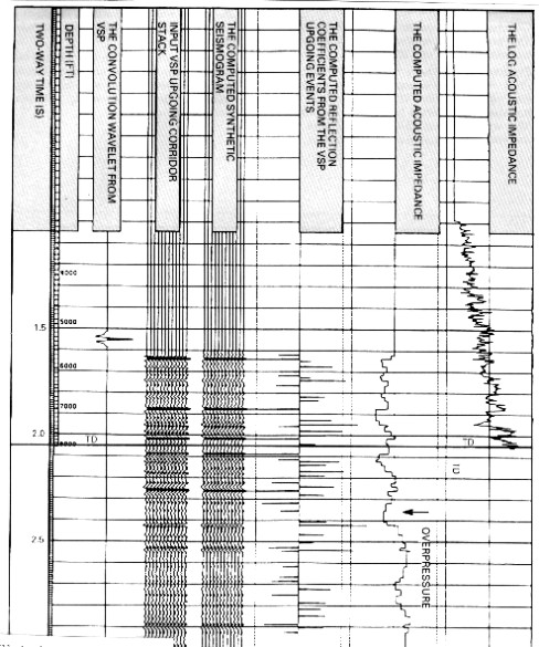
Reservoirs surrounded by these over-pressured shales will also be over-pressured and may cause drilling difficulties or gas kicks into the mud system. At worst, a well blowout may occur. To reduce this risk, it is prudent to review sonic and density logs from offset wells to locate the top of over-pressured zones and use this knowledge to plan drilling and mud programs.

Seismic inversion of vertical seismic profiles can also be used. These are very valuable in the current drilling well since the technique can see a considerable distance below the drill bit. This allows the operator to finetune the estimated depth to top of over-pressure that had been determined earlier from offset wells.

Example of trend lines in a slightly over-pressured shale. Gas kicks occured between 1900 and 2000 feet.

 

VSP, synthetic seismogram, inverted VSP, and original sonic log. Arrow shows overpressure zone on inverted VSP below current drill depth, indicated by  base of sonic log on far right.
 

Calculating Abnormal Pore Pressure
In some reservoirs, pore pressure is higher than normal. These are called overpressured or abnormal pressured zones. The best source of pore pressure is still the extrapolated formation pressures derived from DST or RFT data.

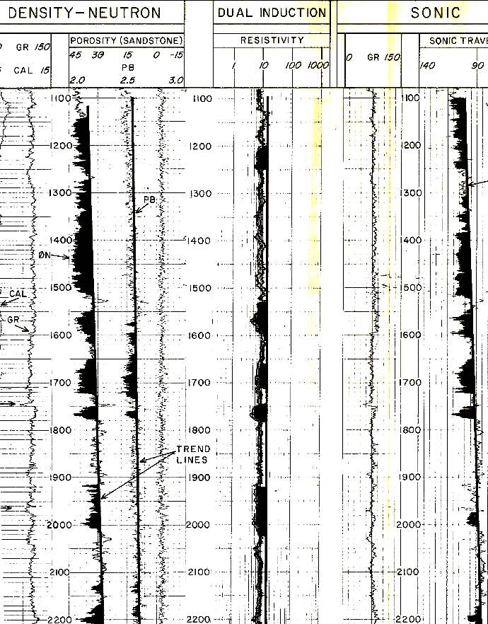
Some gas sands are naturally underpressured due to burial at depth with subsequent formation expansion after surface erosion. There is also some suspicion that glaciation may have pressured then relaxed these zones. Measured pressures are the only source of pressure data for such zones.

Where overpressure data is sparse, a log analysis technique is sometimes helpful. It relies on fitting lines to semi-log plots of sonic travel time in shale versus depth.

First, we need to run a simplified log analysis, just to see where the shales are:
      7: Vsh = MIN(1,MAX(0,((GR - GR0) / (GR100 - GR0))))
      8: PHIe = MIN(PHIMAX*(1 - VSH),MAX(0,0.5 * (PHIN - Vsh * PHINSH + PHID - Vsh * PHIDSH)))

You can substitute a more sophisticated log analysis model if desired. It is used for displaying shale, porosity, and lithology on the depth plot to aid in choosing the normal shale trend line on the sonic log.

Find DTCsh points for the depth plot:
      9: IF Vsh > 0.5 THEN DTCsh = DTC OTHERWISE DTCsh = 0

Fit a best fit or eyeball line to the DTCsh data points (ignoring all zero or null data) above the overpressure zone - this is the normal pressure trend line:
      10: DTCnorm = 10^(log(DTCsh1) - ((DEPTH / DEPTH1) * (log(DTCsh1) - log(DTCsh0))))
      11: DTCdiff = MAX (0,DTCsh - DTCnorm)

Where:
  DTCsh0 = DTCnorm at zero depth
  DTCsh1 = DTCnorm at DEPTH1 on the best fit trend line.

The best fit line through the shale DTC data points define DTCnorm. Equation 10 is an example of such a best fit line. It uses DTCsh0 and DTCsh1 to define the slope of the line. In the example log plot shown a little lower down on this page, DTCnorm is the straight line (on a logarithmic DTC scale) on the left edge of the black shading in the DTC track. The right-hand edge of the black shading is the actual DTC, showing a departure from the trend line towards higher DTC values, thus indicating overpressure.

In equation 10,  DTCsh0 is the extrapolation of the DTCnorm line to zero depth, about 550 - 600 usec/m in this exampl;e. DTCsh1 is picked from the DTCnorm line at DEPTH1, usually at the deepest depth where shale exists in the wellbore.

Calculate overburden pressure gradient from an area specific transform or by integrating the density log:
      12: (Po/D) = (ln (DEPTH - EKB) - 0.5185) / 3.47
      13: Po = (Po/D) * DEPTH

NOTE: All depths must be true vertical depths.

Calculate pore pressure gradient:
      14: (Pp/D) = (Po/D) - ((Po/D) - 1) * (MIN (1 , DTCnorm / DTC))^3
      15: Pp = (Pp/D) * DEPTH

This equation is very sensitive to the choice of the normal trend line. The exponent 3 in the equation may also need adjustment.

CONVERting Pressure TO A "HEAD OF WATER"
Expressed as a “head of water” in meters for hydrodynamic maps:
      16: HEADp = ((Pp/D) - 1) * (DEPTH - EKB)

To convert DST or RFT data to a head of water, rearrange equation 16 to read:
      17: HEADrft = MAX(0,-DEPTH + EKB + RFTPRES / 9.81)

The Pp values from log analysis can be compared to DST or RFT pressures and adjustments made to the best fit lines if needed. There is no good reason to believe that the pressure in a reservoir will be equal to the pressure in the shale above it. However, if a calculated Pp in a shale is less than a measured Pp in a deeper reservoir, then we would expect the formation to leak hydrocarbons or water upward into shallower formations, or even to the surface.

To convert DST or RFT data to a head of water, rearrange equation 10 to read:
      17: HEADrft = MAX(0,-DEPTH + EKB + RFTPRES / 9.81)

EXAMPLE  OF OVERPRESSURE LOG ANALYSIS
An example of this technique is illustrated below.

Overpressure log analysis plot versus depth. Black shading in sonic track indicates overpressure interval. Note that sonic scale is logarithmic and in reverse direction compared to a normal log, and at a highly compressed vertical scale.