CaSE HISTORY - FRACTURED GRANITE Reservoir
Most people forget that there are many unconventional reservoirs in the world, including igneous, metamorphic, and volcanic rocks. Granite reservoirs are prolific in Viet Nam, Libya, and Indonesia. Lesser known granite reservoirs exist in Venezuela, United States, Russia, and elsewhere. Indonesia is blessed with a combination sedimentary, metamorphic, and granite reservoir with a single gas leg. Japan boasts a variety of volcanic reservoirs.

This example is from the Bach Ho (White Tiger) Field in Viet Nam.

Log analysis in these reservoirs requires good geological input as to mineralogy, oil or gas shows, and porosity. A good coring and sample description program is essential, and production tests are essential. The analyst often has to separate ineffective (disconnected vugs) from effective porosity and account for fracture porosity and permeability. All the usual mineral identification crossplots are useful but the mineral mix may be very different than normal reservoirs. Many such reservoirs seem to have no water zone and most have unusual electrical properties (A, M, N), so capillary pressure data is usually needed to calibrate water saturation.

Because the porosity is usually low and mineral mix quite variable, the key to a good fractured reservoir analysis is careful attention to both calculations, as described below.

 

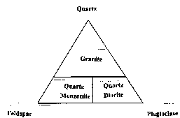
Ternary Diagram for Granite 

In the example below, the granitic mineral assemblage was defined by the ternary diagram at right. The three minerals (quartz, feldspar, and plagioclase) were computed from a modified Mlith vs Nlith model, in which PE was substituted for PHIN in the Nlith equation. If data fell too far outside the triangle, mica was exchanged for the quartz.

Three rock types, granite, diorite, and monzonite, were derived from the three minerals. A trigger was set to detect basalt intrusions. A sample crossplot below shows how the lithology model effectively separates the minerals.

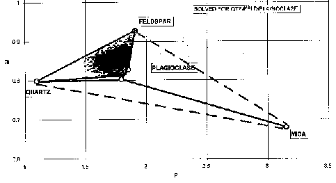
Mlith vs Plith crossplot for granite (micaceous data excluded)

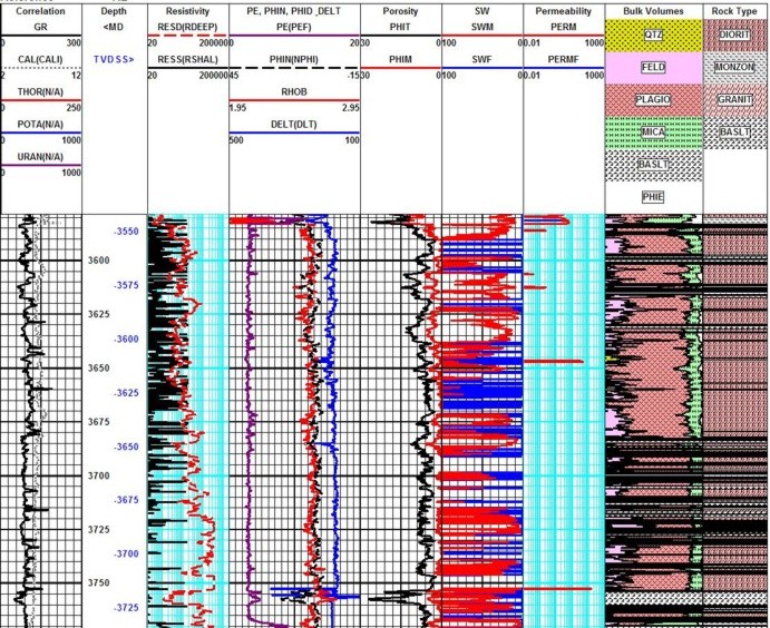
Raw data curves are shown in Tracks 1, 2, and 3 with porosity, water saturation, and  permeability in Tracks 4, 5, and 6. The mineral model calculated from the log analysis is in Track 7 and the rock type model calculated from the minerals using the ternary diagram is in Track 8. Basalt was triggered from high density or high PE or both. Effective porosity (PHIT on log heading) and matrix porosity (PHIM) were calculated from the Aquilera dual porosity model. The difference between them is the sum of solution and fracture porosity.

To test the mineral model and as preparation for calculating the partitioning factor for the dual porosity model, neutron, density, and sonic matrix values, corrected for mineral composition as determined above, were calculated.  Neutron, sonic and density porosity were re-calculated using these matrix values..

Total porosity (PHIt) was taken from the neutron porosity.  Neutron and density were corrected for ineffective matrix porosity, typically 2% for neutron and 5% for density, by comparing log analysis results to available core data. Matrix porosity (PHIm) was then computed from the neutron density crossplot.

Fracture porosity (PHIf) was calculated from the difference between total and matrix porosity. Porosity partitioning coefficient (V) was computed from the ratio of fracture porosity to total porosity. A maximum limit of 0.4% was assumed for fracture porosity. Effective porosity was calculated as the sum of effective matrix and fracture porosity.

Combined M for water saturation (Md) was calculated from the partitioning coefficient and the Aguilera formulae. Fracture water saturation was calculated based on oil and water viscosity and oil formation volume factor. Matrix permeability was calculated from an equation based on core (matrix) porosity versus permeability. Fracture permeability was calculated from fracture porosity assuming a constant aperture of 0.2 mm. 

Fracture porosity from resistivity micro scanner logs was also computed where available to help control the open hole work. A black and white resistivity image log below shows some of the fractures. Both high and low angle fractures co-exist.

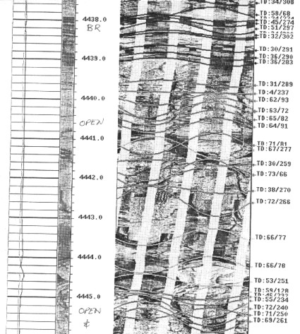
Resistivity micro scanner image in granite reservoir