|
 Log Overlays and Crossplots to Quantify Fractures
Quantitative
fracture methods include fracture intensity calculations that
help to discriminate between lightly fractured and heavily fractured
intervals. Fracture porosity and fracture permeability are covered
as well as secondary porosity index and Pickett plots for finding
the cementation exponent, M.
 Sonic/density
or sonic/neutron porosity overlay presentations help find vugs
and caverns in carbonates. Fractures are often associated with
these porosity types. Sonic derived porosity is generally considered
to be intergranular or intercrystalline (primary) porosity, whereas
density or neutron derived porosity measures primary (intergranular
or intercrystalline) plus secondary (vuggy, solution, or fracture)
porosity. Note that the words primary and secondary porosity are
used here in their traditional log analysis sense and not in a
strict geological sense. However, much of the log analysis literature,
especially with respect to the dual porosity model for fracture
analysis, uses the terms as described in this paragraph. As mentioned
earlier, fracture porosity is very small and is usually overwhelmed
by the vuggy portion. Sonic/density
or sonic/neutron porosity overlay presentations help find vugs
and caverns in carbonates. Fractures are often associated with
these porosity types. Sonic derived porosity is generally considered
to be intergranular or intercrystalline (primary) porosity, whereas
density or neutron derived porosity measures primary (intergranular
or intercrystalline) plus secondary (vuggy, solution, or fracture)
porosity. Note that the words primary and secondary porosity are
used here in their traditional log analysis sense and not in a
strict geological sense. However, much of the log analysis literature,
especially with respect to the dual porosity model for fracture
analysis, uses the terms as described in this paragraph. As mentioned
earlier, fracture porosity is very small and is usually overwhelmed
by the vuggy portion.
Density
neutron crossplot porosity minus sonic porosity yields a result,
traditionally called secondary porosity index or SPI, usually
attributed to vugs or caverns, and to a lesser degree, fractures.
1.
SPI = PHIsec = Max(0, PHIxnd – PHIsc)
Where:
SPI = PHIsec = secondary porosity index
PHIxnd = density neutron crossplot porosity corrected for shale
and lithology
PHIsc = sonic porosity corrected for shale and lithology
The
calculation rules for PHIxnd and PHIsc are defined elsewhere in
this Handbook. Raw logs seldom have the correct scales to make an
adequate overlay, so computer processed curves are usually used.
Lithology must be known or computed accurately for this comparison
to be valid; this is possible in pure limestone sections but not
always in mixed lithology.
If
fracturing is sufficient enough to increase the total porosity
substantially, the porosity comparison method allows fractured
zones to be detected. This is usually not the case, but if an
increase in porosity of more than 1 or 2% due to fracturing is
present, it certainly can be seen.
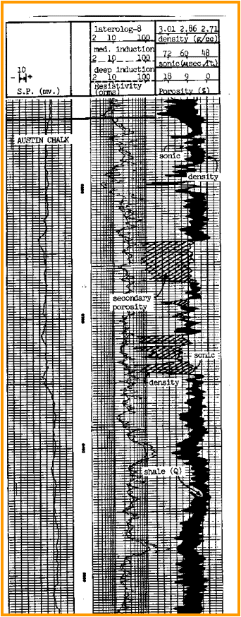 This
illustration shows an Austin Chalk example. The cross hatched area on
the log defines zones where density porosity is greater than sonic
porosity. In this case, it looks like the difference is due to
rough or large borehole, and not entirely to fracture porosity. However,
the presence of fractures is almost certain. This
illustration shows an Austin Chalk example. The cross hatched area on
the log defines zones where density porosity is greater than sonic
porosity. In this case, it looks like the difference is due to
rough or large borehole, and not entirely to fracture porosity. However,
the presence of fractures is almost certain.
 Density - sonic overlay in Austin Chalk Density - sonic overlay in Austin Chalk
A better plot would use the neutron or density neutron crossplot
porosity compared to the sonic porosity, with the sonic porosity
computed with a matrix travel time derived from the density
neutron or density neutron PE lithology calculation. The black
shading shows intervals where density porosity is lower than sonic.
The example claims this is due to shaliness, but some of it may
be due to inadequate lithology compensation in the sonic porosity
calculations.
Methods
have been developed using the above porosity measurements which
lend themselves better to computer analysis. For example, by crossplotting
Mlith and Nlith values, points which fall in certain areas of
the crossplot could represent secondary porosity, ie. vuggy porosity
plus fracture porosity. Secondary porosity raises the Mlith value
compared to the same rock with no secondary porosity.
Other
crossplots using porosity from sonic, neutron, or density versus
each other or gamma ray, and matrix density versus matrix travel
time (MID plot) are also used to solve particular cases. Crossplots
are not as helpful as depth plot overlays.
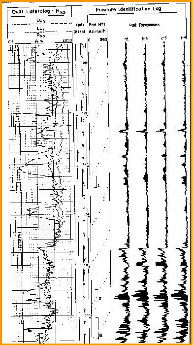 A
deep resistivity/Rxo overlay log is useful in spotting the shallow
resistivity crossover caused by fractures. Rxo is the calculated
value of the formation resistivity with the mud filtrate filling
all pores. The value is derived from the shallowest resistivity
device that was run. This might be a microlog or proximity log,
which are often run on linear scales, making it difficult to compare
to the deep resistivity on a logarithmic scale. Compatible scales
are made in the computer truck or computer center so the analyst
can see what is happening. When Rxo is less than the deep resistivity
in fresh muds, vertical fractures are indicated. A
deep resistivity/Rxo overlay log is useful in spotting the shallow
resistivity crossover caused by fractures. Rxo is the calculated
value of the formation resistivity with the mud filtrate filling
all pores. The value is derived from the shallowest resistivity
device that was run. This might be a microlog or proximity log,
which are often run on linear scales, making it difficult to compare
to the deep resistivity on a logarithmic scale. Compatible scales
are made in the computer truck or computer center so the analyst
can see what is happening. When Rxo is less than the deep resistivity
in fresh muds, vertical fractures are indicated.
Shallow resistivity overlay compared to dipmeter FIL 
Another
approach is to make a crossplot, using logarithmic scales, of
the apparent formation factor against porosity. The plot represents
the Archie formation factor equation:
1.
F = A / (PHIe ^ M) = Rxo / RMF@FT
= Ro / RW@FT
Where:
F = formation factor (unitless)
A = tortuosity constant (unitless)
M = cementation exponent (unitless)
PHIe = effective porosity (unitless)
Rxo = resistivity of invaded zone (ohm-m)
RMF@FT = mud filtrate resistivity at formation temperature (ohm-m)
Ro = resistivity of un-invaded zone water zone (ohm-m)
RW@FT = formation water resistivity at formation temperature (ohm-m)
When
the cementation exponent, M, is a constant it corresponds to a
straight line of constant slope passing through the point F =
A and PHIe = 1.0 on this plot. The tortuosity constant, A, is
often taken equal to 1 for this analysis.
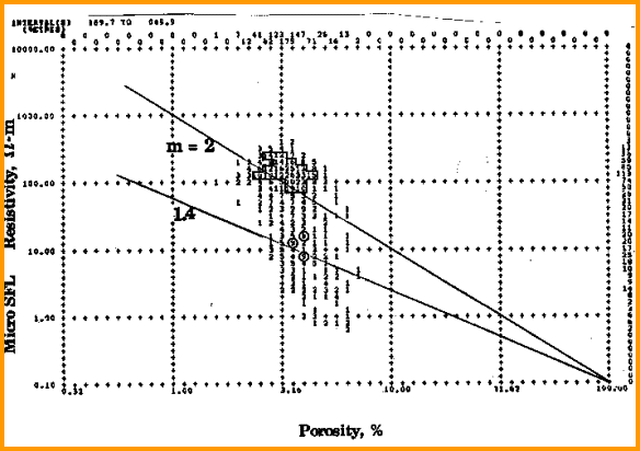
Porosity - resistivity crossplot (Pickett plot)
identifies fractures
In
a non-fractured zone, the apparent M will be slightly too high
if hydrocarbons are present. In a fractured zone, M will be much
lower. Most of the
points in this very tight zone (average porosity = 3%) plot above
the M = 2.0 line due to residual gas saturation. Many points however
plot at much lower values of M and range down to M = 1.1, with
the predominate value near M = 1.4. Low values of M are common
in fractured reservoirs. The more heavily fractured zones give
the lowest M values.
|