|
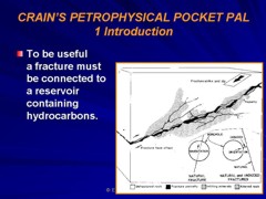
 Fracture Porosity and Permeability From Fracture
Aperture
Fracture Porosity and Permeability From Fracture
Aperture
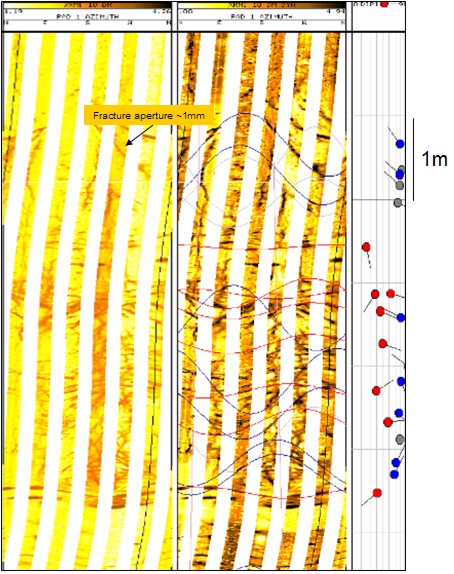
Resistivity
image logs are widely used to assess fracture aperture.
Unfortunately, the image tends to exaggerate fracture aperture,
especially for very small fractures. The fracture noted on the
image at the right looks to be about 1 mm aperture (black streak
on the image). This is about the minimum size that a
fracture can appear on a log because of the pixel density of the
image, electrode spacing on the tool, and erosion of the
wellbore adjacent to the fracture. The fracture frequency may
also be exaggerated if the dip correlation processing picks the
same fracture at different depths. If fracture dios are
hand-picked, fracture frequency will be more accurate.
Fracture aperture exaggeration on acoustic image logs is even more
severe and these logs probably should not be used for aperture
estimation.
These
visual difficulties can be overcome with a post-processing technique
that uses a resistivity inversion model and the mud filtrate
resistivity to calculate aperture, independent of any visual
artifacts.
The algorithm
is based on the concept that higher electrical conductivity means a larger
open fracture. The fracture aperture and fracture frequency can
be combined to obtain fracture porosity and fracture permeability.
1.
PHIf = 0.001 * Wf * Df * KF1
The fracture permeability equations are attributed to Dr Zoltan
Barlai:
2: Kfrac = 833 * 10^11 * PHIfrac^3 / (Df^2 * KF1^2)
3: Kfrac = 833 * 10^5 * PHIfrac * Wf^2
4: Kfrac = 833 * 10^2 * Wf^3 * Df * KF1
 Where: Where:
KF1 = number of main fracture directions
= 1 for sub-horizontal or sub-vertical
= 2 for orthogonal sub-vertical
= 3 for chaotic or brecciated
PHIfrac = fracture porosity (fractional)
Df = fracture frequency (fractures per meter)
Wf = fracture aperture (millimeters)
Kfrac = fracture permeability (millidarcies)
Note:
Equations 2, 3, and 4 give identical results.
Example
1:
Df = 1 fracture per meter
Wf = 1.0 millimeters
PHIfrac = 0.001 * 1 * 1 = 0.001 fractional (0.1%)
Kfrac = 833 * 100 * 1^3 * 1 * 1 = 83300 millidarcies
Example
2:
Df = 10 fractures per meter
Wf = 0.1 millimeters
PHIfrac = 0.001 * 10 * 0.1 = 0.001 fractional (0.1%)
Kfrac = 833 * 100 * 0.1^3 * 10 * 1 = 833 millidarcies
These
examples represent well fractured reservoirs. You can see that
the volume of hydrocarbon is very small but the permeability is
very high.
If
you believe that the phrase “fracture porosity” is
a literal definition, then this porosity will usually be pretty
small - in the order of 0.0001 to 0.01 fractional porosity (0.01
to 1.0%). If you believe that the phrase includes vuggy and solution
porosity related to the presence of fractures, then the value
could be much higher. The important thing is to recognize that
there are two definitions for “fracture porosity”.
An
example of a fracture aperture log from a program called Frac-View
is shown below. The permeability calculation was not
available in this program.
Fracture frequency, aperture, and porosity log derived from
a resistivity image log.
Calculating Permeability From Stoneley Attenuation
 While
propagating along the borehole wall, the Stoneley wave is able
to exchange energy with the formation fluid in a process called
acoustic flow. This communication between the borehole and formation
is proportional to the mobility of the fluids, which in turn is
proportional to permeability and fluid viscosity. Increases in
communication decrease Stoneley amplitude, because energy is used
up when acoustic flow is initiated. This is equivalent to increased
Stoneley attenuation, which therefore can be calibrated to predict
formation permeability. While
propagating along the borehole wall, the Stoneley wave is able
to exchange energy with the formation fluid in a process called
acoustic flow. This communication between the borehole and formation
is proportional to the mobility of the fluids, which in turn is
proportional to permeability and fluid viscosity. Increases in
communication decrease Stoneley amplitude, because energy is used
up when acoustic flow is initiated. This is equivalent to increased
Stoneley attenuation, which therefore can be calibrated to predict
formation permeability.
Permeability from Stoneley wave attenuation 
The
attenuation data can be represented as pseudo-permeability and
presented on a qualitative scale: low attenuation corresponding
to low permeability and high attenuation to high permeability.
To facilitate comparisons of pseudo-permeability to actual formation
producibility, the attenuation data can be integrated to provide
a potential flow profile for comparison to an actual spinner flowmeter
log. .
This
curve could be correlated to core permeability to obtain a calibrated
permeability curve. Correlation is usually as good as porosity
and saturation correlations, which have been used for many years,
and often much better than these in fractured and vuggy zones.
|