PRODUCTION LOGGING BASICS
The primary objective of production logging is reservoir performance evaluation or flow profile evaluation. Production logging is a complex downhole logging technique designed to allow us to determine flowrate, fluid types, and fluid flow distribution in production and injection wells.

Secondary production logging objectives are lift (or completion) performance evaluation and estimations of factors affecting the reservoir performance (leaks and crossflows).

The best known production logging tool is the flowmeter log. There are 3 flavours of flowmeter: continuous or fullbore, diverting, and array spinner flowmeters.

Other measurements are usually needed to aid analysis, including:.
  Temperature log
  Radioactive tracer log
  Noise log
  Focused gamma ray density log
  Unfocused gamma ray density log
  Fluid capacitance log
  Fluid identification log (in high angle wells)
  Gradiomanometer (fluid density) log
  Pressure sensors for static, flowing, build-up, and draw-down pressures
  Gamma ray and collar log for depth control
See links on right-hand navigation menu to access these tool descriptions.

Modern toolstrings include up to one hundred various sensors, and processing techniques utilize probabilistic non-linear algorithms of multiphase flows. The basics are still the same as 40- 50 years ago, but they have been brought into the 21st century..

Production logging is sometimes combined with well integrity logging (multiarm calipers, ultrasonic thickness devices, or serve itself as an indicator with temperature, flowmeter or noise logging sensors) and cased hole formation evaluation logging (multidetector neutron logs, dipole shear sonic logs, pulsed neutron logs with spectrometry capability, natural gamma ray spectrometry logs) in through tubing applications. 

Production logging is usually carried out by the cased hole wireline crew of the service company.  That is carried on wells of different definitions: production wells (on different stage of the field development), injection wells (with water, gas or steam stimulation), exploration wells and wildcats (in combination with conventional DST), hydrology wells and steam energy (geothermal) wells. When the well is producer the test is known as production logging test, when the well is injector – the test is known as an injection logging test.

The number and sequence of production logging tests performed on a well-managed field is defined by the field development team. A good practice is to run the Production Logs at an early stage of the life of the well, in order to establish baseline that will be used later when things go wrong. Too often Production Logs are run when something has gone wrong as the last resort (to design well interventions and workovers or even to take decision to abandon the well).

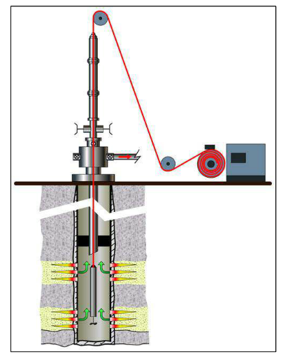
Schematics of Production Logging (KAPPA Eng. DDA handbook)

PLANNING A PRODUCTION LOGGING PROGRAM
A production logging job starts with PL Survey design. A great amount of data is gathered and analyzed. As much data as possible should be taken into account: openhole logs, well integrity logs (CBL’s, Multi-Finger tools, etc), deviation surveys, completion sketches, production (pressures, temperatures, rates), and well intervention history (recent operations). Don't forget the overall geology of the reservoir and detail petrophysical analysis of the porosity, permeability, and saturation profiles relative to the existing completion type and location.

Most modern PLT jobs are run using 2 or 3 different flow rates and several shut-in so as to provide a complete picture of the well's performance capabilities. The main idea is to design a safe, economical, and comprehensive Production Logging Test. 

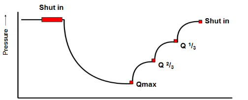
Typical PLT job sequence – flowing regimes and PLT Surveys (marked with red dots). Well flowing rate regime is regulated by the choke size (for natural flowing), gaslift injection rate (for gaslift production), ESP power regulation (electric submersible pump case – in this case special completion solution, known as Y-tool, is required, otherwise logging below the pump is not possible) rod pump power regulation (also special completion solution known as “C-type” annulus is required for logging). For injectors, the situation is the same.  

The above example illustrates 5 PLT surveys being performed (2 in shut in mode and 3 in flowing). Shut in survey (when the well is closed at the surface) is used for downhole tool calibration, pressure estimation, and possible crossflow evaluation.

In well-known fields, the number of flowing regimes may be 2 with no shut in at all. However in exploration wells (or wildcats), I have seen up to 7 flowing regimes with direct and reverse measurements (increasing and decreasing surface rate) and several shut in’s.

In some cases, (low permeability rocks, shale gas formations, etc), the steady state flow cannot be reached (or requires extremely long time for well stabilizing). In this case, the advanced methods, known as isochronal or optimized isochronal tests are being utilized. 

PRODUCTION LOGGING RESULTS
Data processing software takes all the production log sensor information and creates a production profile based on borehole geometry (vertical, deviated, or horizontal) and the fluid phase rates (one, two, or three phases). The math for this is not covered here..

The processed results are the pay zone's phase rate profile (total QZT, interval QZI, relative QZTR) and selective inflow performance SIP diagram.

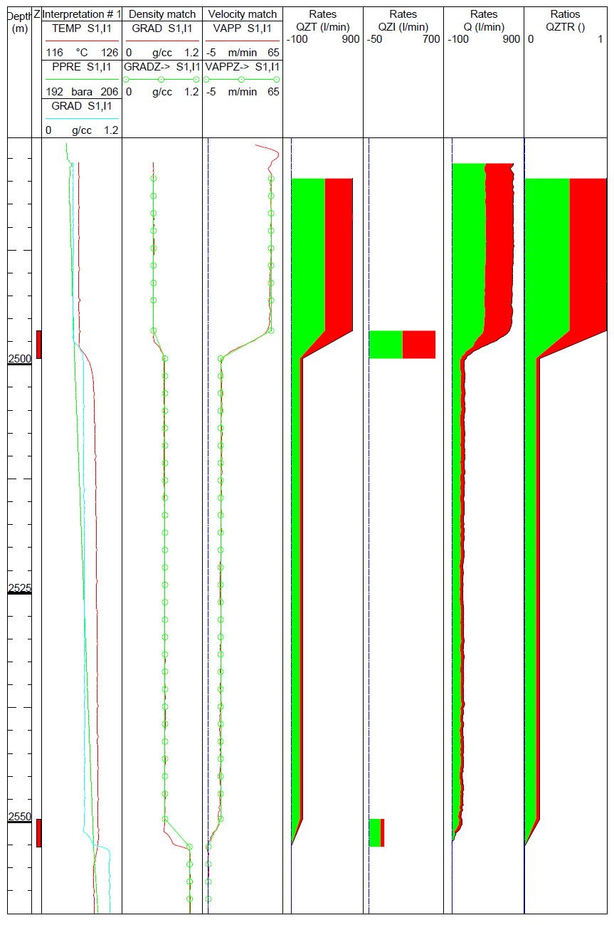
Results presentation of the conventional PLT Survey (Processed with Kappa Emeraude)
Selective Inflow performance (SIP) diagram refers to the pay zone producibility index estimation.
 

The total Inflow Performance Relationship IPR diagram, which is a part of well testing steady state flow data interpretation, reflects the pressure (or dP) as a function of total surface rate.

In contrast, the SIP is constructed for every particular pay zone and flowing phase for  downhole conditions. SIP may be approximated with linear equation, Vogel, Fetkovich or other inflow relationship (like 2,3 – phase or gas inflow cases). The major purpose of this technique is to evaluate the zone rate with particular pressure difference under several conditions.

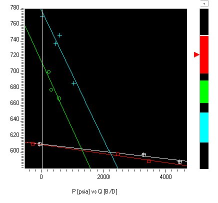
SIP Diagrams (linear approximation for 3 water pay zones with total IPR colored with white – left and Vogel model for 4 oil pay zones below bubble point pressure with total IPR colored with red – right, Kappa Engineering and PetroWiki SPE examples)

SIP is extremely useful reservoir engineering tool that provides an opportunity to estimate reservoir pressure, producibility index, possible zone crossflow and depletion for every pay zone and for various fluid phases. To construct the SIP several well flowing regimes (at least two) are required. Well flowing regime means the well is producing with constant (steady state) or close to steady state at surface. During the PLT, the surface multi-phase rates are measured as usual and are used later for matching with downhole data and velocity (flowing) model

PERMEABILITY FROM FLOW RATE
Once actual flow rate at the formation is determined, reservoir permeability can be calculated.
For linear horizontal flow, Darcy's fluid flow equation relates flow rate to permeability as follows:

      1: Q = 1.127 * A * (K / MU) * (P1 - P2) / L

Where:
  Q = quantity of fluid (bbl/day)
  A = area fluid flows through (sq feet)
  K = permeability (Darcies)
  MU = viscosity of fluid (centipoise)
  P1 - P2 = pressure differential (psi)
  L = length of flow path (feet)

For oilfield work, fluid flow from a reservoir into a wellbore is not linear but radial, so the equation becomes:
      2: Q = 3.07 * H * (K / MU) * (Pr - Pb) / log(Rr/Rb)

Rearranging and solving for K:
      3: K = Q * log(Rr/Rb) * MU / (3.07 * H * (Pr - Pb))

Where:
  K = permeability (Darcies)
  Q = quantity of fluid (bbl/day)
  H = thickness of reservoir that fluid flows through (feet)
  MU = viscosity of fluid (centipoise)
  Pr - Pb = pressure differential from reservoir to wellbore (psi)
  Rr = radius of reservoir = length of flow path (feet)
  Rb = radius of wellbore (feet)

This permeability estimation should be calibrated with other data sources, for example pressure transient analysis technique on pressure buildup or drawdown data, or the geometric average of conventional core analysis data. Some skin-effect  assumptions may be needed.