| 
					
					
					 Case Histories: Synthetic Seismograms Plenty
					of synthetic seismograms have been published in the
					geophysical literature. Here are a few to illustrate the
					variety.
 
 
  Wabamun
                Salt This example is taken from "Geophysical Aspects of Wabamun
                Salt Distribution in Southern Alberta", by N.L. Anderson,
                R.J. Brown, and R.C.Hinds, CSEG Journal, Dec 1988. The example
                shows sonic logs for two wells, one with Wabamun and Cairn salt
                beds, the other without. Both sonic logs have noise and spikes
                which should have been edited.
 
				
				 Wabamun example - raw logs
 
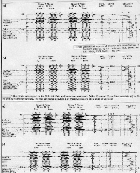
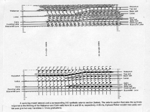
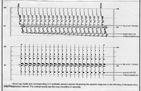
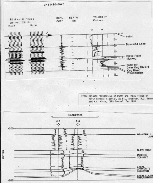
				The
                synthetic (top) shows a model with two salt layers
                based on sonic data only. Adding the density data increases the
                amplitude of the reflections. Comparison of the models make
                it relatively easy to itemize the characteristics of salt and
                salt free cases. Notice that the wavelet frequency is critical
                to identification of the formation tops.  
				
				 Synthetic with salt layer - sonic only (top),
                density added (bottom)
 
				
				 Wabamun example - no salt case
 
				The
				model below portrays a synthetic seismic section based on interpolation
                of the sonic logs between the salt and salt free cases. The model
                would be improved by use of density data augmenting the sonic.
                 
				
				 Wabamun example - synthetic seismic section


			 Swan Hills/Beaverhill Lake (D-3) Reef This model shows the capability of a particular commercially available
                seismic modeling package (GMA). The system takes edited and
				modeled well log data as its basic input. The stratigraphic
				cross section is digitized, along with the log data, or is
				derived from well history data in the data base.
 
				
				 Correlated stratigraphic depth cross section
 
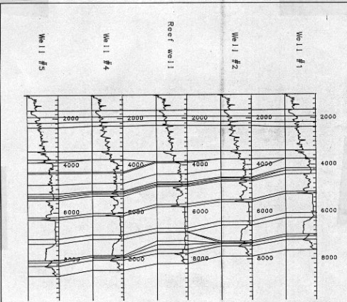
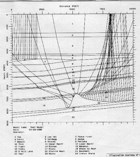
				In
                this example, the reef was edited to a geologically believable
                shape. The acoustic impedance cross section is
                then computed and displayed. This cross section
                uses raw sonic log data that has been interpolated between well
                control. The sonic logs may need editing for bad hole, casing,
                rock alteration, or gas effects. If gas or carbonates are present,
                the model should incorporate density information as well.  
				
				 Edited correlations and hypothetical reef
 
				
				 Acoustic impedance cross section
 
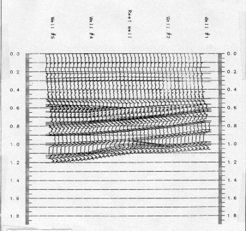
				A
				synthetic seismic section is calculated by creating reflection
				coefficients from impedance and convolving a wavelet with each
				modeled trace.  
				
				 Synthetic seismic section
 
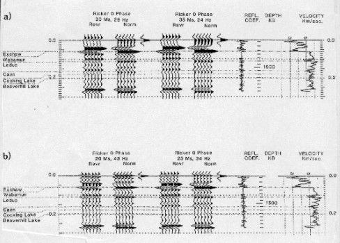
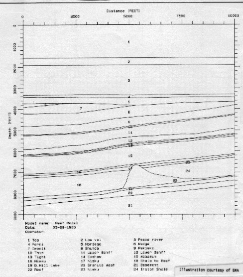
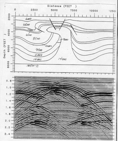
				This
                is the usual form of synthetic modeling, but this example used
                logs which received no editing or correction for invasion. If
                the reef contained gas or had higher porosity than the platform
                rock, the synthetic section would be wrong because the modeled
                velocity and density would be wrong.  
				Thus
                a number of different formation models could be created. The seismic
                response of the models can be compared to each other and to field
                data using discriminant analysis or frequency analysis techniques
                or, more commonly, by visual inspection. If sufficient discrimination
                between various models can be detected, then the comparison of
                these models with field data should provide a valuable interpretation
                aid.  
				Another
                form of modeling is ray path tracing, a time consuming
                computer solution. The ray paths to each key horizon are computed
                from the laws of refraction, and a synthetic section is prepared
                using the noise free reflection coefficients at each layer modeled.
                Both normal (perpendicular) and vertical incidence sections are
                displayed in this example. These are
                used to judge the quality of the reflections to be expected from
                the steeply dipping beds.  
				
				 Ray path tracing on reef model
 
				
				 Synthetic seismic section from ray path tracing
                - normal incidence
 
				
				 Synthetic seismic section from ray path tracing
                - vertical incidence


			 Keg River (Granite Wash) Sand This example is taken from "Seismic Perspective on Panny
                and Trout Fields of North Central Alberta", by N.L. Anderson,
                R.J.Brown, and R.C.Hinds, CSEG Journal, Dec 1989. This example  show sonic log models for a thinning lower anhydrite
                contrasted with a thinning lower clastic. These models help interpreters
                determine which case might be more likely on a seismic section.
 
				
				 Keg River model - thinning anhydrite
 
				
				 Keg River example - thinning sand
 
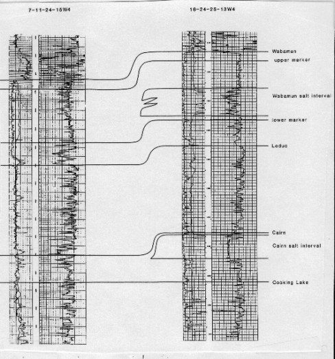
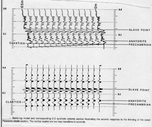
				A
                typical synthetic seismogram is given below as well
                as a geologic cross section from logs. The seismic model, synthetic
                section, and real seismic section follows. The
                basement high and surrounding basal sand are the key elements
                in this model. Note that there is no significant reflection from
                the bald high because the evaporites above mask the event. The
                model would be more realistic if density data were incorporated.
                 
				
				 Keg River synthetic seismograms and log cross
                section
 
				
				 Keg River synthetic section and real seismic
 
                
  More Sophisticated Models Seismic modeling programs can generate the diffraction patterns
                from steep events, so that their interfering effects can be assessed.
                This example shows such a case. Here the diffractions might
                be mistaken for reflection on an anticline instead of the structural
                low that really exists.
 
				
				 Modeling refractions from steeply dipping beds
 
				Stratigraphic
                traps, such as channels, beaches, and bars can also be modeled
                by using adequately modeled log data.  
				
				 Stratigraphic trap model
 
 |