POTENTIAL FIELD DATA REDUCTION AND DISPLAY BASICS
The acquisition of geophysical data such as gravity, magnetic, and radiometric can be accomplished aboard aircraft or ships and on the land surface by survey crews aided by vehicles or helicopters. In addition to the primary measurement, location data and surface elevation are gathered digitally.  The resultant mass of data is most efficiently reduced by using computers with appropriate software, particularly contouring algorithms that can reliably mimic the shapes of subsurface features.

Computer methods also allow a significant amount of further data enhancements to be performed at little additional cost.  Mathematical approaches to estimate regional trends and residual surfaces, continuations and derivatives are the most common.  These mapping functions are also widely used to display formation tops and thickness isopachs, seismic structures and isochrones, and to display the many mappable properties derived from petrophysical analysis (such as pore volume, hydrocarbon pore volume, flow capacity, and net pay)

 This webpage illustrates the results of gravity and magnetic data reduction with a number of examples and workflows, ranging across data acquisition, edit, reduction, and display.

Judicious data edit is the most important factor in obtaining useful exploration information from these computer systems. Editing can be greatly helped by using intermediate maps – bulls eyes or strange kinks in the contours are usually signs of data errors.
 

MAPPING AND CONTOURING METHODS
An overview of a generalized mapping and contouring system is shown in the illustration below.
 

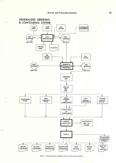
Generalized gridding and contouring system.

 

The essence of digital processing of three-dimensional geophysical or geological data is the interpolation of a numerical surface from the randomly positioned data available after basic corrections and reduction.  This surface is usually sampled at the intersections of a regular square grid, although rectangular or trigonal grids are also used. Once in this grid form, the data may be easily operated on to create new surfaces (e.g. regionals, residuals, continuations, derivatives, isopachs, etc.). The surface is generally displayed in the form of a contour map, although many other displays are possible.

The processing sequence may be broken into four relatively distinct phases: data formatting, numerical surface creation, numerical surface operations, and display. See flow chart above.
 

1)    Data Formatting

 The many different forms of data presented to the system must be placed into a common format after their initial reduction (pre-processing), since the numerical surface creation is a mathematical process independent of the physical meaning of the raw data.  The data must also be sorted on Y co-ordinates within X co-ordinates for the proper functioning of the gridding routines.  This sort and format are the functions of a data preparation program.  It will accept data in almost any form as input and return as output a standard DATA FILE format. 

Naturally, there are utility routines in the systems to operate upon the data file.  Transfer of the file from tape to disc or disc to tape may be necessary.  The contents of the file may be listed with a dump program.  Data records in error or missing may be changed, deleted, or added to the file with a data file update routine.  If the data point locations are not in X-Y co-ordinates, but instead in the form of geographical or survey parameters, another routine must be used to calculate an X-Y map position for every point and create a new data file with this new location information.

A routine should be available to provide a statistical summary of the distribution of the raw data points and recommend a grid interval parameter.  This scan may be useful if the data are fairly randomly distributed such that a good grid interval is not pre-determined by a regular data spacing. 

)   Numerical Surface Creation
Performing the numerical approximation to the surface represented by the data for a regular grid is the function of the next major program.  The usual method used is a plane interpolation and fit that will produce a surface passing exactly through the raw data values.  This is a very critical part of the processing as it must not introduce artificial highs and lows and it must effectively handle edge effects at the boundaries of the map area.  The result is called the GRID FILE. The facility of handling large grids and large numbers of data points through internal segmenting and merge operations is necessary but not many service centers have this ability.  In its absence, the data must be manually segmented with sufficient overlap to avoid ugly anomalies at the joins.  Again, numerous utility routines are usually available to facilitate handling of the GRID FILE.  The transfer of grids from tape to disc or disc to tape is handled as in data preparation.  Errors in individual grid values may be corrected by an update program or a new grid may be created from a subset of an existing grid.  Alternatively, a new grid may be created from an existing grid by halving the grid interval and interpolating new grid points between existing ones.

Should data be already on a grid system but not in the required format, it may be reformatted into a standard GRID FILE for processing in the system by using a program which by-passes the data preparation stage.

Once the desired grid surface has been created many routines exist to perform mathematical operations upon the surface values.

  Numerical Surface Operations
Once a surface exists on a GRID FILE, the user has many options available to help to extract all possible information from his data.  A regional surface for the data may be calculated, either by evaluating a user supplied power series over a grid or by fitting some specified order least squares orthogonal polynomial surface to the data and evaluating either all or some of the resulting co-efficient over the map area.  The order of surface (i.e. the highest power of X and Y) is usually from 2 to 4 to evaluate regional dip and up to 8 or even 16 to evaluate more local anomalies.

The grid surface may be smoothed by a moving quadratic surface, a procedure that is essentially a low-pass filter and may be considered to produce a regional surface if the filter effect is large enough.  Such filtering operations as low-pass, high-pass, strike, continuation and derivatives may be performed by supplying the appropriate co-efficients to a ring operator program.  Filters of completely arbitrary shape and weighting may be designed.

Operations on two sets of grid values such as addition, subtraction, multiplication, division or comparison can then be performed.  For example, residual anomaly maps may be created by subtracting the regional surface from the raw surface.  In addition to ring operator and polynomial surface methods to filter data, Fourier analysis techniques are also available.  This requires considerably more machine time and programming expense as well as a very knowledgeable user, but results are more accurate and have fewer spurious anomalies.

The last option available is usually integration of the surface.  Volume to a bounding plane, surface area or projected area to a plane may be calculated.  This could be of great use in reserves in place calculation.

Having created the desired numerical surface by any suitable means, the user then has available many display options for either line printers or automatic plotters.

)Di Display Options
Certainly the most familiar and quantitatively the most useful means of displaying three dimensional surfaces in a two-dimensional plane is the contour map.  A contour map may be produced for the printer or for a digital or analog plotter.  An extremely useful facility is the ability to produce contour maps in stereographic pairs, which can be a valuable aid to geophysical and geological interpretation.  The user may choose to display his surface as a projection, either in perspective or isometric views.  These types of outputs can be very helpful in showing up trends and linears that may be very hard to identify in an ordinary contour map.

Linear sections of the surface may be taken with a cross section routine.  Profiles such as these are very useful in determining anomaly shapes and sizes and in calculations of such parameters as depth to basement, body size and depth of burial, etc.  This program is also well suited to the display of well information, as many horizons may be plotted for the same section with nearby well control being overplotted on the profiles.

The actual grid values may be posted on the plot, for error checking or hand-contouring.  A similar posting ability exists to output the values from the data file. This again may be done for purposes of error checking; however, the plotter routine more likely will be used prior to hand contouring or for over posting upon a contour map to indicate raw data locations and values.

Finally, as an aid to location of anomalies geographically, a program should be available to generate upon a pre-posted or contoured map or upon an overlay, a grid of geographical co-ordinates.  The co-ordinates may form a Universal Transverse Mercator grid or the major latitude-longitude points on the map sheet.  Clearly, one doesn’t use every program indiscriminately, but chooses a route through the system to optimize data enhancement consistent with the quality of the input data and the processing cost.  In order to make effective use of any of the routines, the input data must be house-cleaned and all basic geophysical or geological corrections made prior to any attempt to contour or analyze the data.  The following section discusses Aeromagnetic and Gravity processing systems as commonly used in petroleum applications.  

AEROMAGNETIC DATA PRE-PROCESSING
The digital processing of aeromagnetic data may also be conveniently broken down and discussed in four phases: data recovery, recovery edit, error correction and mapping.  These phases are basic to the processing of all flight line or discreet point exploration data.  A flow chart of a typical aeromagnetic processing system is shown below.

Data RecoveryThree forms of information may be provided by an aeromagnetic survey.  First, there is of course, the recording of the magnetic value of the earth’s field.  This data is valuable only if properly correlated with the information as to the position of the flight lines along which the data was recorded.  For very accurate surveys, information will also be required on diurnal variations as observed at a fixed ground monitor within the survey area.

The magnetic field values are usually presented to the system as digital values sampled at a constant time increment along the flight line.  The data values at this stage need not occur at integer time values but may be asynchronous to the time (fiducial) count.  Digitally recorded values from the field already satisfy this condition as a rule.  Thus, the only data recovery problem, other than recovery of bad parity or lack of data on tape, will be transcription of the data to cards.  Analog field recordings must be digitized at some convenient sample interval before transcription to cards, by some semi-automatic or manual method.  The values on the cards need not be the true field value, provided the true field may be recovered by simple mathematical operations such as addition or multiplication by a constant.  For card economy, up to 15 values may be transcribed on one card.

The position of a flight line relative to the rest of the survey is generally recovered from a photo mosaic base map with the knowledge of the fiducial count for every given photo center of the mosaic.  If the true geographic position of these photo centres is not directly available, they may be assigned an arbitrary X-Y co-ordinate position relative to some origin and set of coordinate axis.  Thus the position of a flight path may be fully defined by ascertaining the initial and final fiducial values for a line, its direction, and the fiducial values for a line, its direction, and the fiducial count and X-Y position of several photo centres along the flight path.

Information as to the diurnal variation of the earth’s magnetic field may be obtained from the magnitude of the fluctuation of the field as recorded at a fixed ground monitor.  In many cases, this variation is of such a long period that digitizing of this record every several minutes will be sufficient to define the correction required to compensate for this effect.  The system should not require that this monitor be digitized at equal increments in time, so that only major inflections of the record need to be recovered.

Recovery Edit
Once all the data has been recovered in digital form it is important that it be carefully edited to remove the almost inevitable errors in digitizing and transcription.

Since the mapping phase is costly relative to any other phase, reruns caused by correctable data errors can make computer processing of aeromagnetic data uneconomical.

The magnetic field values may be edited by either producing a profile of the line or by scanning the line for point to point variation and proper number of readings. This should point out gross errors in digitizing. Another program should scan the data in standard digitized form for sequential variations in the magnetic field exceeding 100 gammas or some predetermined rate of change and flag such values for possible error.  If the data is synchronous with the fiducial count, a comparison of the number of points expected as calculated from start and end fiducials and the number of data points should point out missing values.

The flight path recovery may be edited by either plotting the flight lines at the same scale as the base map for overlay comparison, or by scanning the fiducial values for proper sequence and the X-Y co-ordinates for expected direction and variance from linearity.

The diurnal data is composed of so few readings that it is probably best edited by hand. 

Error Correction

Assuming that the data has been properly edited for digitizing errors, there remain three major sources of error in the magnetic field values.  These are errors due to diurnal variation in the earth’s field, heading error due to the relation of the flight line bearing to the gradient of the magnetic field, and error due to instrument drift in time.

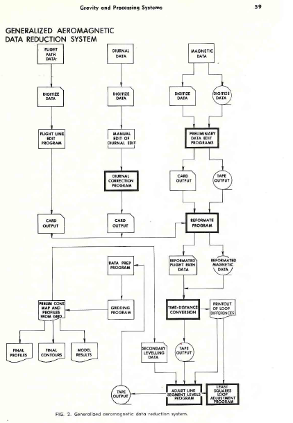
Generalized aeromagnetic data reduction system.

The first correction program calculates the correction required for the first two errors.  It uses the digitized diurnal records to estimate the diurnal correction required at every photo centre, and adds to it a correction for heading error as a cosine function of the flight bearing and a user specified maximum heading error.  A new set of photo centre position data will be created with this correction appended that may be used as input to the next stage. 

Instrument drift will generally be seen as a difference in level between flight lines. 

For short flight lines the drift in a line may be said to be negligible and a bulk correction to each line may be applied to bring the survey to a common datum. If more than one tie line is present, the drift corrections may be made on a time varying basis to adjust the flight lines to the tie lines, assuming accurate recovery of the tie line-flight line intersections. 

Estimation of level corrections in the absence of accurate tie line information requires that the unlevelled data be processed through the mapping phase to a rough grid and contour map.  From this map a region of low magnetic gradient crossing all lines, or several regions covering overlapping groups of lines may be chosen.  Given these regions, profiles perpendicular to the flight lines through the low gradient may be plotted.  If these show oscillation across flight lines dues to levelling error, then the difference between the smoothed and plotted profile at flight line intersections is used as the level correction. 

If good tie line information is available, a least squares network adjustment at flight path intersections can be computed and used as the level correction.  Once the required corrections have been calculated, the magnetic data and positional information is re-formatted into one common form for input to the time to distance conversion program.

This will input the raw magnetic data, photo centre positions and corrections and bulk line level corrections.  The corrections will be applied (interpolated from photo centre corrections) and X-Y co-ordinate positions assigned to each magnetic value and a formatted tape produced.  This output tape is then ready to enter the mapping phase of aeromagnetic processing.

Mapping
The functions of the mapping phase are to interpolate the randomly (almost) distributed data onto a regular grid, if desired perform operations such as two dimensional  filtering or surface operations, and output the data in the form of a contour map, using the mapping system previously described.

GRAVITY DATA PREPROCESSING
Basic gravity data processing to evaluate the Bouguer anomaly is well documented. However, a file oriented system incorporating these calculations with output compatible with a standard gridding, contouring and evaluation system is not always available.  A flow chart of such a system is shown in the image below.

In a typical system, the Bouguer anomaly is calculated first, in the following steps:

1)    Drift correct elevation data from barometric readings or loop tie vertical survey data.

2)    Calculate latitude and longitude of stations from survey data.

3)    Build data file of raw data (meter readings, barometric readings, location co-ordinates, time, station number).

4)    Using known base stations, apply drift correction to gravity data.

5)    Calculate and apply meter corrections, latitude corrections, elevation corrections (water depth and Eotvos corrections if data from ship borne survey).

6)    Output to data file.

From there, various utility routines must be available to print results by loops or by station numbers, to update a file or abstract a portion of a file, and to change the Bouguer density without recomputing the entire survey.

Terrain corrections may be necessary and this may be facilitated by the computer in one of two ways.  One approach is to enter the evaluations of each segment of the Hammer chart for each station and allow the computer to calculate, sum, and apply the terrain effect of all segments.  This method is the cheapest and most effective if station spacing is far apart (e.g. 4 - 6 km), and elevation control is poor.

Where elevation control is very good and station spacing is close (e.g. 250 – 500 ft), the method normally used is to digitize the elevation data on a grid about the same size as the data spacing.  The gravitational effect of each prism, bounded by the grid lines is computed and added to the Bouguer value at the station.  Due to the number of computations involved, it may be necessary to interpolate a finer grid near the station and group prisms together farther from the station to obtain a compromise between accuracy and computing time.

The output from any of these options can then be entered directly into the gridding and contouring system for display and analysis. The most common results desired, aside from the Bouguer anomaly map, are profiles perpendicular to strike or anomaly axis and regional and residual surfaces.  The profiles are often matched to synthetic models by successive approximation or else an iterative curve fitting routine is applied which varies the depth, orientation, and density contrast of some postulated causative body until a reasonable fit to the observed profile is found.

There is no doubt that computer methods in gravity data reduction can assist by providing accuracy, speed, and a master file which simplifies subsequent work.  There is no doubt either that unless the user is very careful at the data collection and editing stage, they can eliminate all these advantages by allowing the programs to operate on erroneous data.  Because errors are easily found and corrected while computing and contouring by hand, it is sometimes difficult to get used to the idea that the machine can’t do this.  All it can do is flag suspicious results and wait for assistance.  But, if the test for suspiciousness is not subtle enough, the test may pass erroneous data, to be discovered later by the interpreter as a rather “ungeologic” anomaly on a final computer contoured map.

It cannot be emphasized enough that error detection and correction are the most important part of all these systems and cannot be done without intelligent people interacting with well-designed programs.

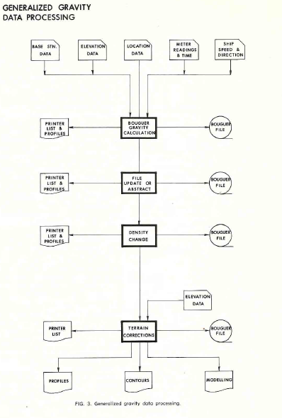
Generalized gravity data processing.

GRAVITY DATA REDUCTION MATH
Data reduction of large amounts of land or marine gravity data can be accomplished with a program especially designed  to handle the variety of location, elevation, or water depth data, as well as tables of gravity meter constants. Meter drift, loop and line tie differences and running average filters can be applied.  Results of free air and Bouguer corrections are output to a file, which can be updated, or used as input to computer contouring or profile routines. 

The mathematical formula used for the corrections are as published by Grant and West in “Interpretation Theory in Applied Geophysics” published by McGraw-Hill, 1956.  

For land-based gravity surveys, these are:

     1.  G = 978049.0 * (1 + 0.005 288 4 * Sin² L – 0.000 005 9 Sin²L)

     2 . E = 0.09416 – 0.00090 * Cos (2*L) – 0.068 * 10^-7  * H

     3.  B = -0.01276 * DENS * H

     4.  T = 0.005 * Ts * DENS

Where:

          G = theoretical gravity at latitude L

          E = elevation correction at latitude L for elevation H

          B = Bouguer correction for replacement density DENS

               T = terrain correction for T value of Ts at 2.00 g/cc for replacement
                density DENS

The Bouguer Anomaly is:

     5.  BG = Observed Gravity + E + B + T – G

For marine gravity surveys (moving platform), the equations are:

     6. G = As above

     7. B = 0.01276 * (DENS – DENSW) * W

     8. E = 7.5074 * V * Cos L * Sin A –  0.004 16 * V^2

Where:

          B = Bouguer correction for replacement density DENS and water density
           DENSW * water density for water at depth W

          E = Eotvos correction for ship speed V at latitude L with course direction A

The Bouguer Anomaly is:

     9.  BG = Observed Gravity + B + E – G

The units of measurement used in the equations are as follows:

          G = milligals

          L i= degrees from Equator

          H = feet

          DENS = grams per cubic centimeter

          DENSW = grams per cubic centimeter

          Ts = gravity units (0.10 milligal)

          W = feet

          V = Knots

          A = degrees from true North

If anyone can provide equations in Metric Units, please contact me.


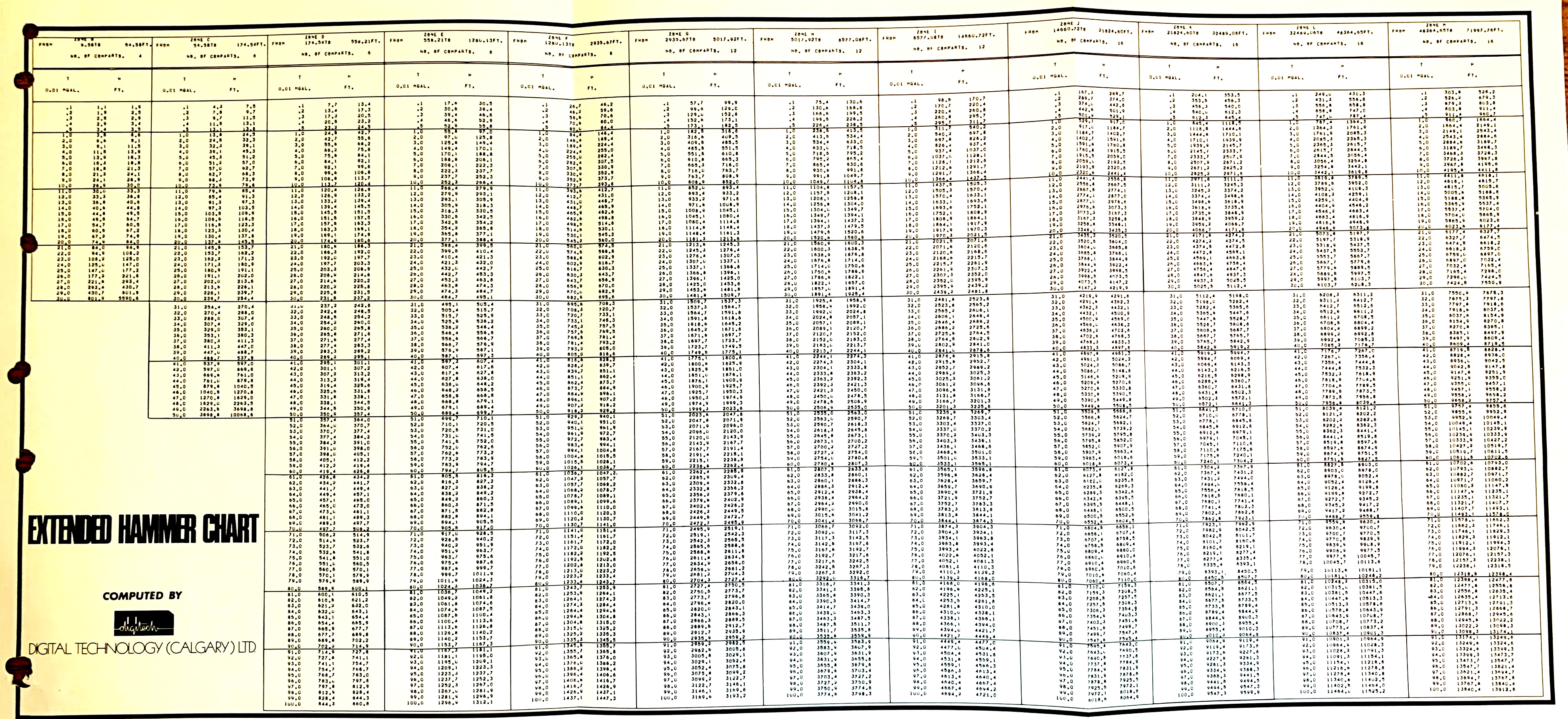
EXTENDED HAMMER CHART FOR TERRAIN CORRECTIONS
Manual calculation of terrain corrections was tedious and made use of a shortcut called the Hammer Chart. It was first publishes as “Terrain Corrections for Gravimeter Stations” by Sigmund Hammer, Geophysics Vol. IV, No. 3 (1939) pp 184 – 194.

These early versions of Hammer Charts for computation of terrain corrections for gravity data have been limited in their range of elevations, T-values, and radii. In 1973,a computer program was developed to compute extended tables of the standard form to any value of T and to any radius. The attached chart is representative of the results computed to a T value of 100 (where possible).

Download large scale image (3900x1800px) of the sample Extended Hammer Chart

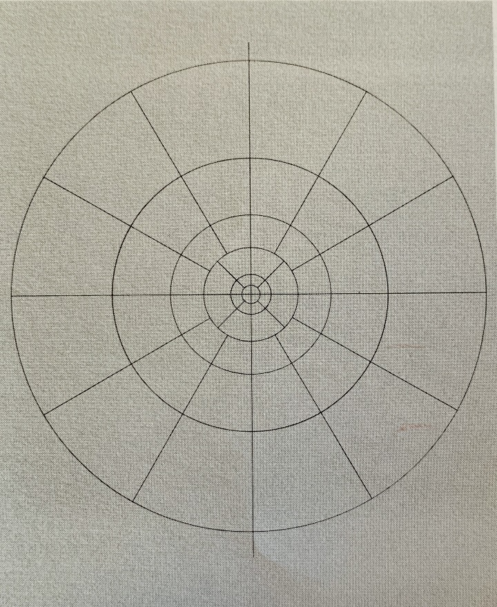
Schematic diagram of elevation cylinders for terrain corrections using Hammer’s method

The formula used for the computation is from Sigmund Hammer’s1939 paper. as shown below:

Extended Hammer Equation.

 Where:

          Hj = height of cylindrical segment of one compartment which produces a gravity effect  .g₀

          R₁ = inner radius of zone

          R₂ = outer radius of zone

          a = ratio of outer to inner radius

          n = number of compartments in the zone

          g₀ = 10^⁵ gals.

          y = 6.670 * 10^⁸ dyne cm2 / gm2

          j = any positive number

          rho = rock density (2.00 gm/cc assumed)

This formula is exact and not the first few terms of a series expansion.

Nomograph for Hammer Chart Calculations.

 

MAPPING EXAMPLES
This Section will discuss various examples with the view to showing the following:

1)    Machine contour quality is satisfactory for a great many applications.

2)    Regional-residual analysis using polynomial or smoothed surfaces can aid in the identification of significant anomalies.

3)    That just like manual contouring, every contour package will produce slightly different maps, given the same input data and the same control parameters.

EXAMPLE 1: Formation Tops
The first example, shown in below (3 images) consists of posted well top data for one horizon, with a third order trend (regional) surface, and the residual after removal of the trend.  As we can see, the regional dip is to the west-southwest at the rate of about 50 feet to the mile.  The residual anomaly map clearly shows closed highs and lows relative to the regional dip, and if we refer to the posted map, most of the wells will be found on the up dip (NW) side of these high closures.  If an explorationist intended to recommend another well, it would be useful to have such a set of maps to assist in picking the correct location.  It is unfortunate that the usefulness of such a map is directly proportional to the number of wells already drilled, so that when we need it most we can’t make it due to lack of control.

Posted and contoured well-top data.

Third order trend (regional) surface of well-top data.

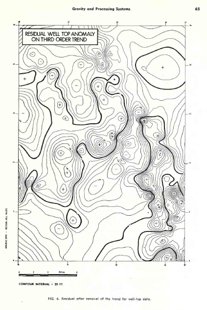
Residual after removal of the trend for well-top data.

EXAMPLE 2: Aeromagnetic Survey
The second example is from a portion of an aeromagnetic survey, shown below (5 images).  This is a highly complex intrusive in a fairly flat regional and in order to look at small anomalies which may be of interest a low pass filter was applied and subtracted from the data to give the residual.  Some linear features running north-south and the east-west  faults cutting them are more clearly defined on the residual, although they were visible on the original map.

Other display forms, such as the perspective view, and the flight line profiles are useful in visualizing the total magnetic intensity surface and should assist in interpretation by considering anomaly shapes.

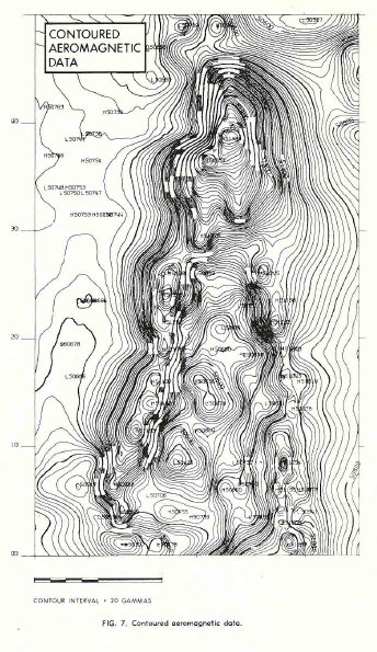
Contoured aeromagnetic data.

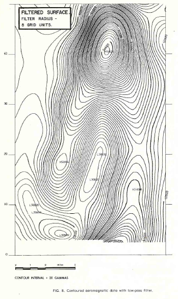
Contoured aeromagnetic data with low-pass filter.

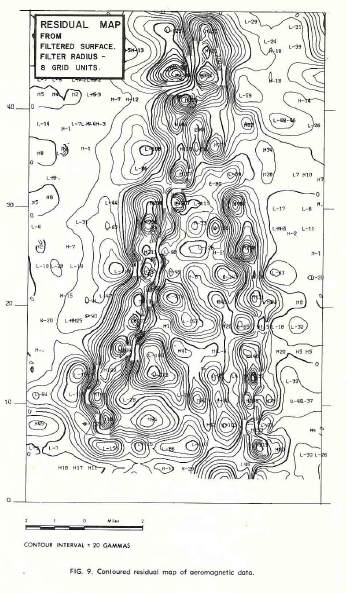
Contoured residual map of aeromagnetic data.

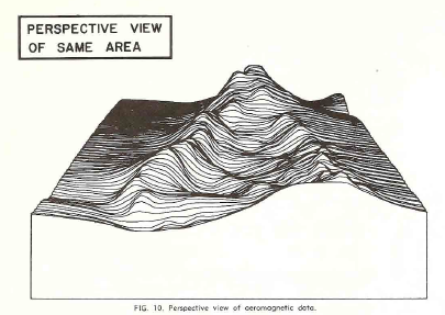
Perspective view of aeromagnetic data.



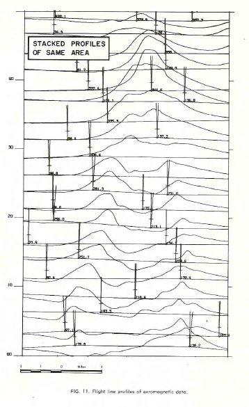
Flight line profiles of aeromagnetic data.

EXAMPLE 3: Gravity Data
The third example represents a portion of a gridded gravity survey of the Bouguer anomaly, shown below (3 images).  Again, a regional surface was removed and a residual map reflecting the closures on the regional was created.  The residual is only 2.0 milligals so the data reduction and editing prior to mapping were obviously important.

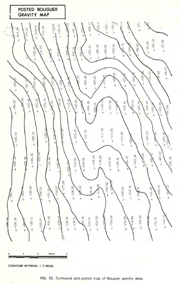
Contoured and posted map of Bouguer gravity data.

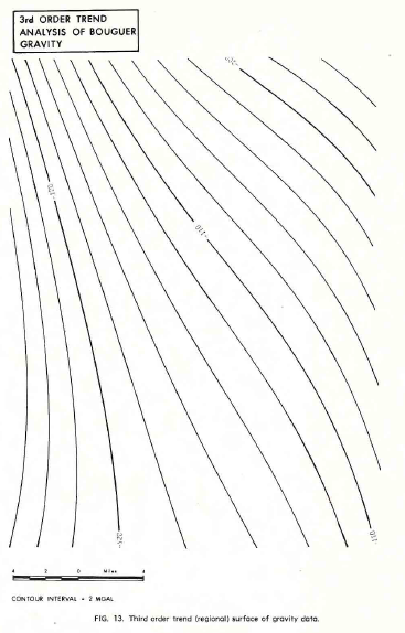
Third order trend (regional) surface of gravity data.

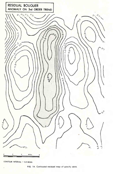
Contoured residual map of gravity data.