WATER ANALYSIS METHODS
Laboratory water analysis is an essential measurement required for accurate water saturation calculations from log data. Water samples are collected from drill stem tests or produced fluids. In the case of produced fluids, the water should be captured from the flow line and separated later from the oil. Samples from separators or treaters may not be representative of formation water due to contamination. Samples from drill stem tests are usually taken at the top, middle, and bottom of the test recovery. The bottom sample should have the least contamination from drilling fluid invasion. The top sample will have the most contamination.

Laboratories usually measure from 9 to 15 of the individual ions in a water sample, recorded in milligrams/litre (mg/l) or grams/cubic meter (g/m³). These two sets of units are equivalent: 1 mg/l = 1 g/m^3.  At low to moderate concentrations, one mg/l is very close to 1 part per million (ppm) so mg/l and ppm tend to be used interchangeably. The difference is that ppm = mg/l divided by the density of the water.

In older reports, results were quoted in grains per gallon (gpg)  One grain per US gallon equals 17.1 mg/l or approximately 17.1 ppm. 

The cations (positive ions) are measured by ion chromatograph. These are Sodium (Na), Potassium (K), Calcium (Ca), Magnesium (Mg), Iron (Fe), and sometimes Barium (Ba), Strontium (Sr), or Boron (Bo). The anions (negative ions) cannot be measured by ion chromatograph so Chloride (Cl) and sometimes Iodide (I) and Bromide (B) are still measured by titration. Bicarbonate (HCO₃) and Carbonate (CO₃) are calculated from the volume of acid required to reduce the pH to 8.3 (for CO₃) and 4.5 (for HCO₃). Sulphate (SO₄) is calculated by adding a volume of Barium Chloride and then measuring the turbidity of the solution. The sum of all of these measured ions becomes the calculated total dissolved solids (TDS).

They also measure, in a routine analysis, the pH, relative density, and resistivity (Rw) of the water sample.  The Rw is measured in ohm-m and they will record the temperature at which it was measured. This temperature will be used to adjust the measured Rw to a common "laboratory temperature", usually 25 Celsius or 77 Farenheit. Some labs use different standard temperatures.

Some labs also provide mmol/l (or moles/m³).  mg/l (or g/m³) divided by the molar mass of the ion equals mmol/l (or moles/m³). Since mg/l is the same thing as g/m³, mmol/l is the same thing as mol/m³. Molar mass is derived from the atomic weight of the ion on the Periodic Table. For instance, the atomic weight of S is 32 and the atomic weight of O is 16, so the molar mass of SO₄= 32 + 4 * 16 = 96.

Most labs calculate milli-equivalents (MEQ).  MEQ equals mmol/l or moles/m³ multiplied by the valence or charge of the ion.  SO₄ has a negative charge of 2 so 1 mmol/l of SO₄ equals 2 MEQ of SO₄.  Sodium (Na) has a positive charge of 1, so 1 mmol/l of Na equals 1 MEQ of Na. 

The logging company charts that convert ppm to Rw are based on ppm of pure NaCl. This is because the most common formation waters found in the world are NaCl based. These charts will give you the wrong Rw if the fluid is a mud filtrate which is mostly Na₂SO₄ or if the fluid is Sodium Bicarbonate type formation water.

The diagram at the bottom of the water analysis is called a Stiff Diagram. It is a graphical representation of the different ions.  The shape of the Stiff Diagram can become a “fingerprint” which can allow us to distinguish whether the fluid is formation water or an introduced fluid, and can often distinguish the zone from which the formation water was produced.

SAMPLE WATER ANALYSIS REPORT

Water analysis report from a drill stem test recovery, showing chemical analysis, calculated and measured water resistivity, and Stiff diagram of chemical analysis. This is a fairly salty formation water with salinity of 146,000 parts per million (ppm) and a resistivity of 0.066 @ 25C.

WATER SAMPLE CONTAMINATION
Contamination of water samples by drilling fluid invasion is common and the Stiff Diagram helps to spot this problem. For instance, a typical gel-chem type mud filtrate recovery will have Na in MEQ divided by Cl in MEQ of 5 or greater. Most contamination problems require some experience and a supply of Stiff Diagram fingerprints that are reasonably consistent. For more information on fingerprinting water recoveries, please contact Opus Petroleum Engineering Ltd., www.opuspetroleum.com.

The Canadian Water Resistivity Catalog is well screened, but field samples may be contaminated. The following rules of thumb are useful in detecting mud filtrate contamination or meteoric water recharge.

   1. Mg/l and ppm are approximately the same thing except in very saline waters.

   2. Most gel-chem mud filtrates are usually from 3000 to 8000 mg/l TDS.

   3. When the log header says gel-chem mud, they might mean gyp’ed-up mud. Gyp’ed-up mud usually has soda ash added to compensate for drilling through anhydrites. Gyp’ed-up mud filtrates are usually from 10,000 to 25,000 mg/l TDS.

   4. KCl mud filtrates are usually from 30,000 to 50,000 mg/l TDS with lots of K and lots of Cl.

   5. Potassium Sulphate mud filtrates are usually from 50,000 to 80,000 mg/l TDS with lots of K and lots of SO4.

   6. Salt-saturated mud filtrates are usually 300,000 mg/l or higher.

   7. Generally speaking, formation waters increase in salinity with depth but see #12.

   8. Each zone should have a unique formation water “fingerprint” or Stiff Diagram unless it is hydraulically connected to another zone.

   9. This formation water “fingerprint” may change with location in the basin.

   10. Most formation waters have a milli-equivalent Na/Cl ratio of 0.6 to 1.2.

   11. Many formation waters are fresher than expected as they are affected by fresh water recharge from the surface. These recharge waters have a distinctive fingerprint which is high in bicarbonates and the milli-equivalent Na/Cl ratio is usually between 2 and 3. These fresh waters have been found in formations as deep as the Devonian and can under-run more saline formation waters.

   12. Never rely on one water analysis as being representative of the formation water in a particular pool and field. Try to find at least three water samples in your pool that have formation water characteristics, are close to the same TDS and have similar “fingerprints”. Then compare the Rw on your samples to the ones in the catalog.

Agat Lab in Calgary uses a "Smart Chart", incorporating these rules,  to help identify clean water samples from those contaminated by mud filtrate or other chemicals.

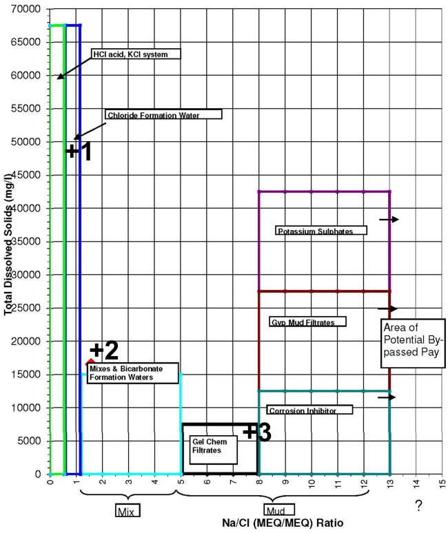
This crossplot of TDS versus the Na/Cl ratio helps check for contamination. Data point 1 is in the formation water category. Point 2 is either naturally high in bicarbonates or contaminated by some gyp-based mud invasion. Point 3 is mostly gel-based mud filtrate.
 

 Equivalent NaCl Water Salinity from Water Analysis
The resistivity of a water sample can be calculated from its chemical analysis. To do this, an equivalent NaCl concentration must be determined based on the ionic activity of each ion.

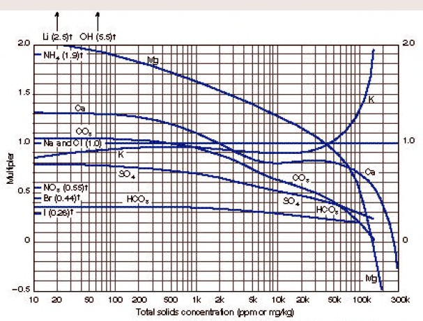
Enter chart with total solids concentration of the sample in ppm (mg/kg) to find weighting factors for each ion present. The concentration of each ion is multiplied by its weighting factor, and the products for all ions are summed to obtain equivalent NaCl concentration.
 

The math is pretty simple:
      1: TDS = SUM (IONi)
      2: WSe = SUM (IONi * FACTRi)

Where:
  TDS = total dissolved solids (ppm)
  IONi = ion concentration of ith component (ppm)
  FACTRi = multiplier factor for ith component (ppm)
  WSe = equivalent NaCl concentration (ppm)

NUMERICAL EXAMPLE:
Assume formation-water sample analysis 
  460 ppm Ca,
  1400 ppm SO4 
  19,000 ppm Na plus Cl.

Total dissolved solids concentration
  TDS = 460 + 1400 + 19,000 = 20,860 ppm
Entering the chart with this total solids concentration
  Ca multiplier = 0.81
  SO4 multiplier = 0.45
  Na+CL multiplier = 1.00
Equivalent NaCl concentration = 460 ´ 0.81 + 1400 ´ 0.45 + 19,000 ´ 1.0 = 20,000 ppm.

Water Salinity from Chloride Content
Sometimes salinity is reported at the well site in ppm Chlorides instead of ppm NaCl equivalent.
      6: WSa = Ccl * 1.645

Where:
Ccl = water salinity (ppm Cl)
WSa = water salinity (ppm NaCl)

COMMENTS:
Use this relationship when chloride content of the water sample is known. Usually Cl content is derived at the well site from a drill stem test recovery. It is useful as a first approximation until the water sample is analyzed more accurately at a laboratory. The relationship is for pure NaCl solutions and the factor may be higher or lower if other ions are present.

NUMERICAL EXAMPLE:
1. Chloride concentration to salinity.
WS = 11,600 ppm Cl * 1.645 = 19,000 ppm NaCl

Water Resistivity from Salinity AT ANY TEMPERATURE
Crain's Model is used to convert a lab measured salinity to a formation water resistivity (RW) at any specific temperature (FT) in degrees Fahrenheit. The result is abbreviated as RW@FT throughout this Handbook. You can use equation 5 to convert a salinity to any arbitrary temperature, for example 75F or 77F (roughly 25C) to find the resistivity at laboratory conditions.
      1: FT = SUFT + (BHT - SUFT) / BHTDEP * DEPTH
      2: IF LOGUNITS$ = "METRIC"
      3: THEN FT1 = 9 / 5 * FT + 32
      4: OTHERWISE FT1 = FT
      5: RW@FT = (400000 / FT1 / WS) ^ 0.88

SALINITY FROM WATER RESISTIVITY
Invert Crain's equation to solve for WS given RW at a a specific temperature FT1.
      6: WS = 400000 / FT1 / ((RW@ET) ^ 1.14)

Where:
  BHT = bottom hole temperature (degrees Fahrenheit or Celsius)
  BHTDEP = depth at which BHT was measured (feet or meters)
  DEPTH = mid-point depth of reservoir (feet or meters)
  FT = formation temperature (degrees Fahrenheit or Celsius)
  FT1 = formation temperature (degrees Fahrenheit)
  RW@FT = water resistivity at formation temperatures (ohm-m)
  SUFT = surface temperature (degrees Fahrenheit or Celsius)
  WS = water salinity (ppm NcCl)

COMMENTS:
Use this relation if salinity is known from laboratory measurements to obtain RW from lab data at any temperature.

NUMERICAL EXAMPLE:
1. Salinity to water resistivity.
RW@FT = (400000 / 102'F / 20,000 ppm) ^ 0.88 = 0.238 ohm-m @ 102'F
(rounded to three significant digits)

2. Water resistivity to salinity.
WS = 400,000 / 102'F / ((0.250 ohm-m) ^ 1.14) = 19,000 ppm NaCl
(rounded to three significant digits)

Water Resistivity from Salinity at Lab Temperature
These models generate RW at laboratory temperature of 75F or 25C.
Crain's Method (1974)
     1: RW@75F = (400000 / 75 / WS) ^ 0.88

Bateman and Konen Method (1977)
     2: RW@75F = 0.0123 + (3647.5 / WS^0.955)

Kennedy's Method (2015)
     3:  RW@75F = 1 / (24.30853 - 0.0364 * (0.1 * WS - 29.46515957) - 0.02922 * (0.1 * WS - 29.46515957)^2)

SALINITY FROM WATER RESISTIVITY
Crain's Method (1974)
      4: WS = 400000 / 75 / ((RW@75) ^ 1.14)

Baker Atlas Method (2002)
      5: WS = 10 ^ ((3.562 - (Log (RW@75 - 0.0123))) / 0.955)

COMMENTS:
For all practical purposes, the three models give the same RW value (see Graph 1 below). There are minor differences above 150,000 ppm NaCl which can only be seen when water resistivity is converted to water conductivity (see Graph 2 below).

The effect on water saturation (SW%) is not very significant (+/- 0.5% SW at low SW, +/- 2% SW at high SW, at 200,000 ppm NaCl).

The 10 significant digits used in the Kennedy equation give a false sense of accuracy that is not warranted.

Graph 1: Rw Models - Red line = Crain, Black line = Bateman and Konen, Blue line = Kennedy


Graph 2: Cw Models - Red line = Crain, Black line = Bateman and Konen, Blue line = Kennedy.
The differences above 150,000 ppm NaCl have little impact on water saturation. 

NUMERICAL EXAMPLE:
   
 

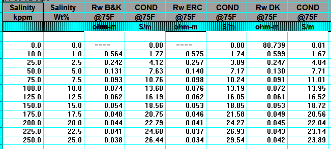
  RW from  Water Catalogs
Water catalogues published by your local well logging society or similar catalogues created by searching in-house data bases are a necessary tool for well log analysis. A sample is shown below.

A sample of RW data from a water resistivity catalog, data is tabulated and also
 posted on a map, and is based on a standard temperature of 25 degrees Celsius (77 degrees Fahrenheit).

Water resistivity values in a catalog are recorded at a standard temperature, usually 75F or 77F (25C). Since water resistivity varies inversely with temperature, the catalog values must be transformed to a new value representing water resistivity at formation temperature (RW@FT) -- see next Section.

To use data from a water catalogue, it is usually necessary to do a little filtering. Nearly everything that can go wrong will raise the RW value recorded in the catalogue. Usually the minimum value from nearby offset wells is the best choice. It may be useful to gather all the values for the reservoir for a radius of 3 to 6 miles (5 to 10 Km) and prepare a histogram. On the histogram, find the point that represents the lower decile (10% of the data values are less than this value). Take the average of the data in this decile. You may want to eliminate obvious "impossible" values before you make the histogram.

The following relationships are needed to manipulate water resistivity data prior to calculations of water saturation.
1. Arps Method (1953)
      1: FT = SUFT + (BHT - SUFT) / BHTDEP * DEPTH
      2: KT1 = 6.8 for English units    KT1 = 21.5 for Metric units
      3: RW@FT = RW@TRW * (TRW + KT1) / (FT + KT1)
      4: RMF@FT = RMF@TRW * (TRW + KT1) / (FT + KT1)
      5: RMC@FT = RMC@STRW + (TRW * KT1) / (FT + KT1)

Where:
  SUFT = surface temperature for temperature gradient (degrees Fahrenheit or Celsius)
  BHT = bottom hole temperature (degrees Fahrenheit or Celsius)
  BHTDEP = depth at which BHT was measured (feet or meters)
  DEPTH = mid-point depth of reservoir (feet or meters)
  FT = formation temperature (degrees Fahrenheit or Celsius)
  RMC@FT = mud cake resistivity at formation temperature (ohm-m)
  RMC@TRW = mud cake resistivity at surface temperature (ohm-m)
  RMF@FT = mud filtrate resistivity at formation temperature (ohm-m)
  RMF@TRW = mud filtrate resistivity at surface temperature (ohm-m)
  RW@FT = water resistivity at formation temperatures (ohm-m)
  RW@TRW = water resistivity at surface temperature (ohm-m)
  TRW = temperature at which water was measured (degrees Fahrenheit or Celsius)

2. Hilchie Model (1984) ALL temperatures in Fahrenheit.
      6: KT1 = 10^ ( --0.340396 * log(RW@TRW) + 0.641427)
      7: FT1 = SUFT + (BHT - SUFT) / BHTDEP * DEPTH
      8: RW@FT = RW@TRW * (TRW + KT1) / (FT1 + KT1)
      9: RMF@FT = RMF@TRW * (TRW + KT1) / (FT1 + KT1)
      10: RMC@FT = RMC@STRW + (TRW * KT1) / (FT1 + KT1)

Where:
  FT1 = formation temperature (degrees Fahrenheit ONLY)

COMMENTS:
Use these relations when RW@TRW is known from measured data. This transformation can be made on the chart below. The Hilchie model accounts for the slight curvature at low and high temperatures on the chart, but Arps model is quite sufficient for practical petrophysics.

NUMERICAL EXAMPLE:
1. Water resistivity at formation temperature.
English units example:
RW@FT = (0.32 ohm-m @ 77'F) * (77 + 6.8) / (102 + 6.8) = 0.25 ohm @ 102'F

Metric units example:
RW@FT = (0.32 ohm-m @ 25'C) * (25 + 21.5) / (39 + 21.5) = 0.25 ohm-m @ 39'C

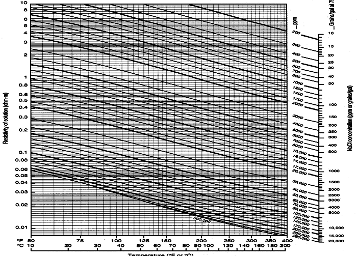
Schlumberger Chart GEN-9: Water resistivity - Temperature - Salinity relationships

 ESTIMATING SURFACE AND FORMATION TEMPERATURES
Temperature measurements specific to your area of interest are going to sparse and you will have to do some searching for useful data. The map below gives a good idea of what to use for surface temperature (SUFT). Temperature versus depth data from log headings can be plotted to estimate a best fit temperature gradient line. It doesn't have to be a straight line. See representative graphs below. In areas with sparse data, use the temperature gradient maps supplied below.

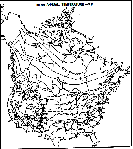
Mean Annual Surface Temperature Map for North America - degrees F
The 40 deg F contour follows roughly along the US-Canada border except along the coast lines.
Contour interval is 5 deg F.

Typical Depth - Temperature profiles. Create your own by best fit of BHT vs BHTDEP from data on log
 headings or DST reports.

Temperature gradient for USA - degrees Celsius per 1000 meters,
North American Heat Floe Map (3 MB)    Legible Legend for NA Map

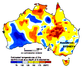
Temperature at 5000 meters for Australia

  META/LOG "RW" SPREADSHEET -- Water Resistivity Calculations
This spreadsheet calculates RW at formation temperature using 5 different methods.

Download this spreadsheet:
SPR-07 META/LOG WATER RESISTIVITY (RW) CALCULATOR
  Calculate water resistivity (RW), 5 methods,
 

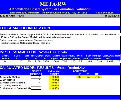
Sample of "META/RW" for calculating water resistivity from various methods.