fractured reservoirs
The other Sections of this Chapter showed numerous examples of individual fracture location techniques. The case histories shown here show examples of projects that may use more than one technique, or amplify the use of a single technique in a unique environment. Study these six examples for the subtle clues that help identify fractures on open hole logs.

A Classic Example
This example consists of a very complete set of older logs, all of which show a short fractured zone at 376-381 m. This is the best you will get in older wells before the era of image logs. If you are chasing tight gas, tight oil, or shale gas, you will need to be competent at recognizing all the clues. See if you can spot all the fracture indicators before reading on.










 

Open hole logs for A Classic Example

Dipmeter log for A Classic Example

The deep resistivity curve has a clear conductive anomaly showing that at least some of the fractures appear to be sub-horizontal with respect to the well. The shallow resistivity is affected the same way. The dual laterolog and Rxo log curves are also affected. The Rxo reading is very low. Because the shallow resistivity is lower than the deep, fractures are indicated. Mud resistivity is too fresh for this to be a salt mud invasion phenomenon.

The density and neutron logs show a high porosity zone while the density correction is very hashy.

The sonic log is strongly affected by cycle skipping. The waveforms on the sonic variable intensity display practically disappear. The sonic amplitude curve is very low. The caliper may be suggesting some mud cake, while the GR log indicates some radioactivity, probably due to uranium salt accumulation in the fractures.

Finally, the dipmeter fracture identification log clearly shows the fractures as individual anomalies. Six different anomalies can be defined; some probably are sub-horizontal. Very short vertical fractures are also present. There was a serious loss of circulation opposite this zone when the well was drilled.

Austin Chalk Example
Logs from 3 different Austin Chalk wells are shown in here. They all demonstrate the typical Austin Chalk pattern of heavy fractures near the top of the zone, grading to few fractures near the middle. The amount of fracturing does vary considerably between wells. This can be seen by the different amount of activity on the dipmeter curves and is also reflected in the initial production of the wells.

Dipmeter curves for Austin Chalk Example

Dipmeter curves presented in Fracture Identification Log (FIL) format show fractured intervals. The well on the right has far fewer fractures than the well shown on the left.

Austin Chalk fractures can be oriented by using the dipmeter azimuth to determine the direction of hole diameter elongation. A frequency plot of fracture orientations from wells in the Pearsall Field area, have an average strike of N 39 E with a range from N 13 E to N 57 E.

Reservoir development proceeded by orienting large fractures in the good wells or in offset wells where a dipmeter was run. New locations were drilled along these joint lineations. Where an offsetting good well had no available dipmeter data, an average orientation value was used appropriate for that area. Well potentials and production records substantiate the success of this method.

Fractured Shale Example
This is a comparison of logs over a section of the upper Miocene fractured shale from Kern County, California. This section is noted for its high apparent porosities (40%) and low permeabilities. Fractures are required for it to be productive. The interval was conventionally cored through the top 20 feet (6.1 m) of zone. The core was described as shale, thinly laminated and fractured parallel to low angle bedding planes.

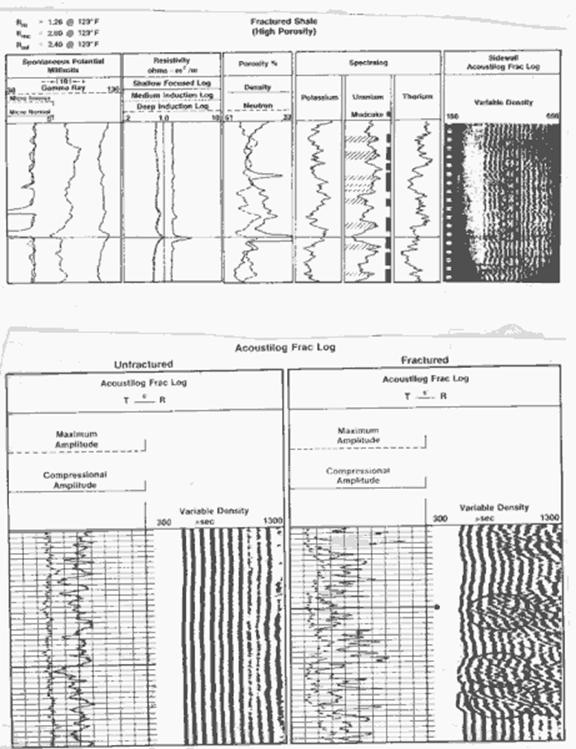
Open hole logs for Fractured Shale Example

The SP, gamma ray, microlog, dual induction focused log, density, neutron, gamma ray spectral log, and sidewall acoustic log from this well are shown above. The resistivity measurements show low resistivity and straight line character. The SP did develop and has the same approximate character as the gamma ray.

The gamma ray spectral log provides the most character through the section. The method of analysis of the spectral log curves is to look for intervals which have low values of potassium and thorium. These are zones with less clay minerals, possibly less plastic and more receptive to fracturing. In these zones, present or past permeability is indicated by a higher uranium content. Several such intervals exist and correlate with zones on which mudcake formed indicating present permeability. Intervals which show the higher uranium with lower potassium and thorium have been marked with black bars. They are the most likely to produce.

The sidewall acoustic variable density log is typical of a high porosity sequence. Intervals on the log show high compressional amplitude and reduced shear amplitude, indicating low angle fractures. A few intervals illustrating this response are circled. Chevron patterns are faintly.

A portion of un-fractured log is shown opposite a fractured section for comparison in the bottom half of the above illustration. Notice the different character between the compressional amplitude and the variable intensity display. The chevron patterns are quite distinct.

Formation Micro-Scanner in Fractured Shale

The formation micro-scanner image of a similar fractured shale is shown above. Notice the steep dips, fine bedding, and the fracture. The sand/shale ratio can be determined easily by computer processing of the image.

Vertical Fracture in Vertical Hole
This example shows a modern televiewer log over a portion of a hole with a vertical fracture intersecting the borehole. The image is displayed as a 360 degree unwrap with East at the center of the image, and as an equivalent core image, with South in the middle.

Acoustic televiewer in vertical fracture, vertical hole

Notice the enlarged borehole in some of the thin shale beds. The fracture plane is far from smooth and it wanders from one side of the borehole to the other. A dipmeter or older FMS might miss this fracture, or indicate discontinuous vertical fractures. Light colors are higher acoustic impedance, probably dolomite versus darker colored limestone and limey shales. Shale beds are black and washed out.

Vertical Fracture in Horizontal Hole
Here a drill pipe conveyed televiewer was run over a 1500 foot horizontal stretch from the intermediate casing shoe. The zone is an upper Cretaceous chalk in which fractures play a vital role in productivity. Most vertical wells penetrate only one or two fractures and deplete quickly. A horizontal well can penetrate many fractures and production can be significantly enhanced.

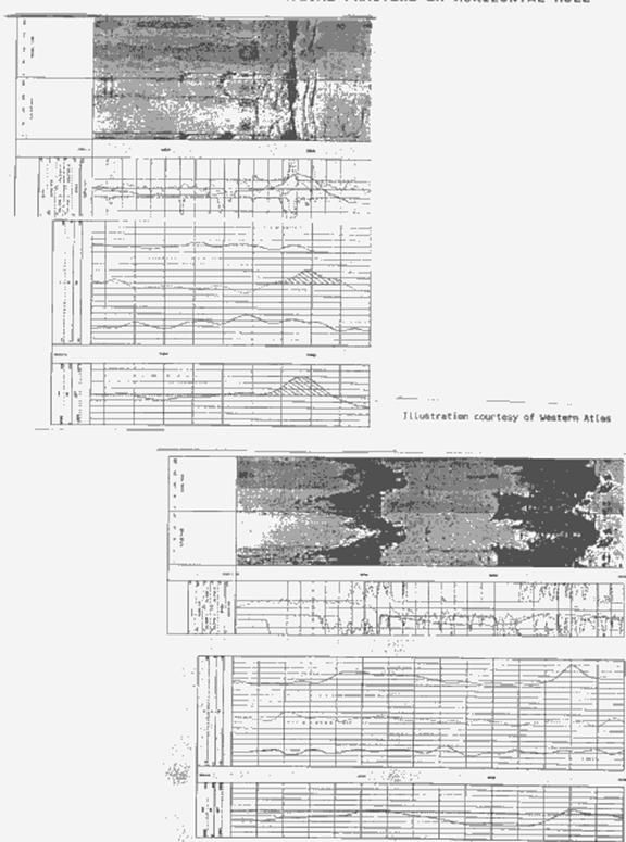
Acoustic televiewer in vertical fracture, horizontal hole

The televiewer images and uranium precipitation shown on the spectral gamma ray log indicate fractures clearly. This allows the operator to position completion hardware, such as centralizers and external inflatable casing packers correctly. In this example, the hole was designed to run close to the top of the chalk, and it penetrated the marly zone above in a few places, shown by the dark bands. It sometimes helps to look at these images horizontally when analyzing horizontal wells. Both acoustic amplitude and acoustic travel time images are presented side by side. The black sinusoidal patterns are wider than the actual fractures as this is a pretty old version of the logging tool - a more modern log would do a better job than this.